X
wikiHow is a “wiki,” similar to Wikipedia, which means that many of our articles are co-written by multiple authors. To create this article, 11 people, some anonymous, worked to edit and improve it over time.
This article has been viewed 216,570 times.
Learn more...
Hiding rows and columns you don't need can make your Excel spreadsheet much easier to read, especially if it's large. Hidden rows don't clutter up your sheet, but still affect formulas. You can easily Hide and Unhide rows in any version of Excel by following this guide.
Things You Should Know
- Highlight the rows you wish to hide. Then, right click them and select "Hide".
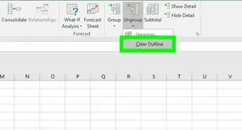
- Create a group by highlighting the rows you wish to hide and going to Data > Group. A line and a box with a (-) should appear. Click the box to hide the grouped rows.
- Unhide by highlighting the rows above and below the hidden cells, right clicking, and choosing "Unhide". Alternatively, hit the (+) sign next to the rows if it is available.
Steps
Method 1
Method 1 of 2:
Hiding a Selection of Rows
-
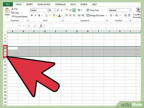
1Use the row selector to highlight the rows you wish to hide. You can hold the Ctrl key to select multiple rows.
-
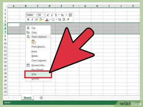
2Right-click within the highlighted area. Select “Hide”. The rows will be hidden from the spreadsheet.Advertisement
-
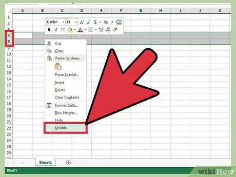
3Unhide the rows. To unhide the rows, use the row selector to highlight the rows above and below the hidden rows. For example, select Row 4 and Row 8 if Rows 5-7 are hidden.
- Right-click within the highlighted area.
- Select “Unhide”.
Advertisement
Method 2
Method 2 of 2:
Hiding Grouped Rows
-
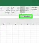
1Create a group of rows. With Excel 2013, you can group/ungroup rows so that you can easily hide and unhide them.
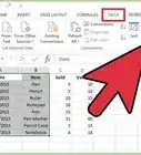
- Highlight the rows you want to group together and click "Data" tab.
- Click "Group" button in the "Outline" Group.
-
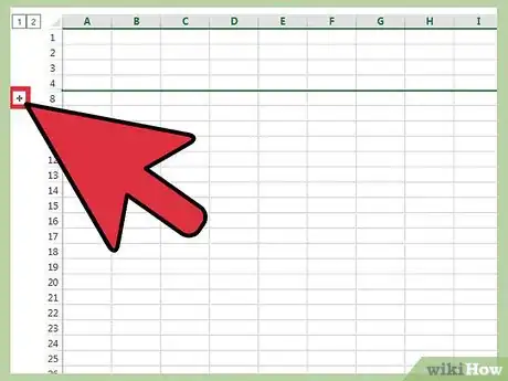
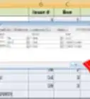
2Hide the group. A line and a box with a (-) minus sign appears next to those rows. Click the box to hide the "grouped" rows. Once the rows are hidden the small box will display a (+) plus sign.
-
3Unhide the rows. Click (+) box if you want to unhide the rows.
Advertisement
Community Q&A
-
QuestionWhat if the hidden rows were 123 in Excel?
 Community AnswerJust select the cell or cells, then go to Home, and in Cells group, click Format. Then under Visibility, point to Hide\Unhide, and then click Hide Rows or Hide Columns. This will hide the Rows or Columns of the selected cell or cells.
 -
QuestionHow do I hide non-consecutive rows containing a specific word in a given column?
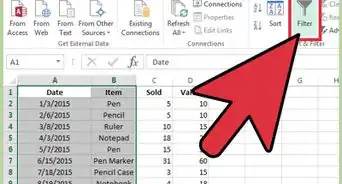
 Community AnswerHighlight the entire spreadsheet. Go to Data then click on Filter. This will add a drop-down box in the header of each column. Click on the drop-down box in the column where the specified words you want to hide is located. De-select all of the items you wish to hide, and click OK.
 -
QuestionWhat is the purpose of hiding rows?
 Community AnswerHiding rows you don’t need can make your Excel spreadsheet much easier to read, especially if it’s large. For example, if you want to input data that is used for multiple formulas, a hidden row will still contain that information but will not be shown.
Advertisement
About This Article
Article SummaryX
1. Select rows to hide.
2. Right-click the highlighted area.
3. Click Hide.
Did this summary help you?
Advertisement
