How to Use AutoFilter in MS Excel

Co-authored by wikiHow Staff

Last Updated: October 6, 2021

Excel's AutoFilter features makes it quick and easy to sort through large quantities of data. We'll show you how to use both pre-set and custom filters to boost your productivity in Excel in no time!

Part 1

Part 1 of 2:

Getting Started with AutoFilter

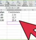
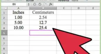
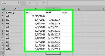
1
Create a table. Make sure that your data have column headings to specify the data below it. The heading is where the filter will be placed and will not be included in the data that is sorted. Each column can have a unique dataset (e.g. date, quantity, name, etc.) and contain as many entries as you wish to sort through.
- You can freeze your headings in place by selecting the containing row and going to “View > Freeze Panes”. This will help keep track of filtered categories on large data sets.
2
Select all the data you wish to filter. Click and drag to select all of the cells you wish to be included in the filter. Since AutoFilter is, as the name implies, an automatic process, you cannot use it to filter non-contiguous columns. All columns in between will be set to filter with them.

Advertisement
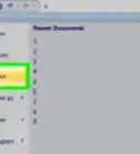
3
Activate AutoFilter. Go to the “Data” tab, then press “Filter”. Once activated, the column headers will have drop-down buttons. Using these buttons, you can set your filter options.
4
Select filter criteria. Filters options can vary based upon the type of data within the cells. Text cells will filter by the textual content, while number cells will have mathematic filters. There are a few filters that are shared by both. When a filter is active a small filter icon will appear in the column header.
- Sort Ascending: sorts data in ascending order based on the data in that column; numbers are sorted 1, 2, 3, 4, 5, etc. and words are sorted alphabetically starting with a, b, c, d, e, etc.
- Sort Descending: sorts data in descending order based on the data in that column; numbers are sorted in reverse order 5, 4, 3, 2, 1, etc. and words are sorted in reverse alphabetical order, e, d, c, b, a, etc.
- Top 10: The first 10 rows of data in your spreadsheet or the first 10 rows of data from the filtered selection
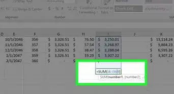
- Specific conditions: Some filter parameters can be set using value logic, like filtering values greater than, less than, equal to, before, after, between, containing, etc. After selecting one of these you will prompted to enter the parameter limits (e.g. After 1/1/2011 or greater than 1000).
- Note: the filtered data is hidden from view, NOT deleted. You will not lose any data by filtering.

Part 2

Part 2 of 2:

Customizing and Deactivating Autofilter

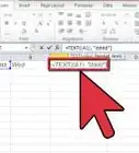
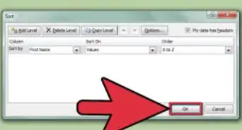
1
Utilize custom AutoFilter for more complex sorting. A custom filter allows for multiple filters to be applied using “and/or” logic. The “Custom Filter…” option is listed at the bottom of the filter dropdown menu and brings up a separate window. Here you can select up to two filter options, then select the “And” or “Or” button to make those filter exclusive or inclusive.
- For example: a column containing names could be filtered by those containing “A” or “B”, meaning Andrew and Bob would both appear. But neither would appear in a filter set for those containing both “A” and “B”.
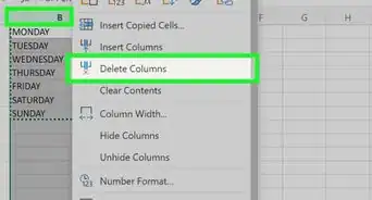
2
Clear your filters. To clear a single filter, select the dropdown for the filtered column and select “Clear Filter From [name]”. To clear all filters, select any cell in the table and go to the “Data” tab and press “Clear” (next to the Filter toggle).
3
Deactivate AutoFilter. If you want to disable the filters completely, simply deselect the AutoFilter option while the table is selected.

Community Q&A

Question

How do you know when the autofilter is turned on?

Community Answer

Dropdown menus will appear at the top of each column. Those with active filters will display a small filter icon next to the dropdown menu arrow.
Question

Not all the variables in my field of data are appearing in my filter selection. How do I correct this?

Community Answer

It's possible that you have set conflicting filters. Try clearing some of your filters. If you are using a custom filter, check your "and/or" logic.
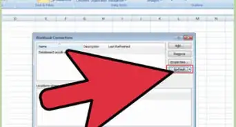
Question

How can I set Excel 2007 so that upon opening, AutoFilter will have the "select all" box to be unchecked?

Community Answer

This checkbox cannot be deselected by default. If you use Advanced Filter instead of AutoFilter, you can select which ranges you want filtered from the start.

Warnings

By filtering your data, you are not deleting rows, you are hiding them. Hidden rows can be unhidden by selecting the row above and below the hidden row, right-clicking on them and selecting "Unhide".

⧼thumbs_response⧽
Helpful 5 Not Helpful 2
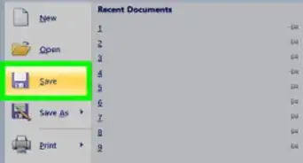
Save your changes frequently unless you have backed up your data and are not planning to overwrite your data.

⧼thumbs_response⧽
Helpful 5 Not Helpful 2