This article was co-authored by wikiHow staff writer, Jack Lloyd. Jack Lloyd is a Technology Writer and Editor for wikiHow. He has over two years of experience writing and editing technology-related articles. He is technology enthusiast and an English teacher.
This article has been viewed 1,898,162 times.
Learn more...
One of the best features of Excel is its ability to calculate your mortgage-related expenses like interest and monthly payments. Creating a mortgage calculator in Excel is easy, even if you're not extremely comfortable with Excel functions. This tutorial will teach you how to create a mortgage calculator and amortization schedule in Microsoft Excel.
Steps
Creating a Mortgage Calculator
-
1Open Microsoft Excel. If you don't have Excel installed on your computer, you can use Outlook's online Excel extension in its place. You may need to create an Outlook account first.
-
2Select Blank Workbook. This will open a new Excel spreadsheet.Advertisement
-
3Create your "Categories" column. This will go in the "A" column. To do so, you should first click and drag the divider between columns "A" and "B" to the right at least three spaces so you don't run out of writing room. You will need eight cells total for the following categories:
- Loan Amount $
- Annual Interest Rate
- Life Loan (in years)
- Number of Payments per Year
- Total Number of Payments
- Payment per Period
- Sum of Payments
- Interest Cost
-
4Enter your values. These will go in your "B" column, directly to the right of the "Categories" column. You'll need to enter the appropriate values for your mortgage.
- Your Loan Amount value is the total amount you owe.
- Your Annual Interest Rate value is the percentage of interest that accrues each year.
- Your Life Loan value is the amount of time you have in years to pay off the loan.
- Your Number of Payments per Year value is how many times you make a payment in one year.
- Your Total Number of Payments value is the Life Loan value multiplied by the Payments Per Year value.
- Your Payment per Period value is the amount you pay per payment.
- Your Sum of Payments value covers the total cost of the loan.
- Your Interest Cost value determines the total cost of the interest over the course of the Life Loan value.
-
5Figure out the total number of payments. Since this is your Life Loan value multiplied by your Payments Per Year value, you don't need a formula to calculate this value.
- For example, if you make a payment a month on a 30-year life loan, you would type in "360" here.
-
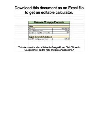
6Calculate the monthly payment. To figure out how much you must pay on the mortgage each month, use the following formula: "= -PMT(Interest Rate/Payments per Year,Total Number of Payments,Loan Amount,0)".
- For the provided screenshot, the formula is "-PMT(B6/B8,B9,B5,0)". If your values are slightly different, input them with the appropriate cell numbers.
- The reason you can put a minus sign in front of PMT is because PMT returns the amount to be deducted from the amount owed.
-
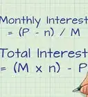
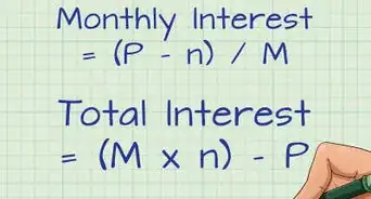
7Calculate the total cost of the loan. To do this, simply multiply your "payment per period" value by your "total number of payments" value.
- For example, if you make 360 payments of $600.00, your total cost of the loan would be $216.000.
-
8Calculate the total interest cost. All you need to do here is subtract your initial loan amount from the total cost of your loan that you calculated above. Once you've done that, your mortgage calculator is complete.


Making a Payment Schedule (Amortization)
-
1Create your Payment Schedule template to the right of your Mortgage Calculator template. Since the Payment Schedule uses the Mortgage Calculator to give you an accurate evaluation of how much you'll owe/pay off per month, these should go in the same document. You'll need a separate column for each of the following categories:
- Date - The date the payment in question is made.
- Payment (number) - The payment number out of your total number of payments (e.g., "1", "6", etc.).
- Payment ($) - The total amount paid.
- Interest - The amount of the total paid that is interest.
- Principal - The amount of the total paid that is not interest (e.g., loan payment).
- Extra Payment - The dollar amount of any extra payments you make.
- Loan - The amount of your loan that remains after a payment.
-
2Add the original loan amount to the payment schedule. This will go in the first empty cell at the top of the "Loan" column.
-
3Set up the first three cells in your "Date" and "Payment (Number)" columns. In the date column, you'll input the date on which you take out the loan, as well as first two dates upon which you plan to make the monthly payment (e.g., 2/1/2005, 3/1/2005 and 4/1/2005). For the Payment column, enter the first three payment numbers (e.g., 0, 1, 2).
-
4Use the "Fill" function to automatically enter the rest of your Payment and Date values. To do so, you'll need to perform the following steps:
- Select the first entry in your Payment (Number) column.
- Drag your cursor down until you've highlighted to the number that applies to the number of payments you'll make (for example, 360). Since you're starting at "0", you'd drag down to the "362" row.
- Click Fill in the top right corner of the Excel page.
- Select Series.
- Make sure "Linear" is checked under the "Type" section (when you do your Date column, "Date" should be checked).
- Click OK.
-
5Select the first empty cell in the "Payment ($)" column.
-
6Enter the Payment per Period formula. The formula for calculating your Payment per Period value relies on the following information in the following format: "Payment per Period<Total Loan+(Total Loan*(Annual Interest Rate/Number of Payments per Year)),Payment per Period,Total Loan+(Total Loan*(Annual Interest Rate/Number of Payments per Year)))".
- You must preface this formula with the "=IF" tag to complete the calculations.
- Your "Annual Interest Rate", "Number of Payments per Year", and "Payment per Period" values will need to be written like so: $letter$number. For example: $B$6
- Given the screenshots here, the formula would look like this: "=IF($B$10<K8+(K8*($B$6/$B$8)),$B$10,K8+(K8*($B$6/$B$8)))" (sans the quotation marks).
-
7Press ↵ Enter. This will apply the Payment per Period formula to your selected cell.
- In order to apply this formula to all subsequent cells in this column, you'll need to use the "Fill" feature you used earlier.
-
8Select the first empty cell in the "Interest" column.
-
9Enter the formula for calculating your Interest value. The formula for calculating your Interest value relies on the following information in the following format: "Total Loan*Annual Interest Rate/Number of Payments per Year".
- This formula must be prefaced with a "=" sign in order to work.
- In the screenshots provided, the formula would look like this: "=K8*$B$6/$B$8" (without quotation marks).
-
10Press ↵ Enter. This will apply the Interest formula to your selected cell.
- In order to apply this formula to all subsequent cells in this column, you'll need to use the "Fill" feature you used earlier.
-
11Select the first empty cell in the "Principal" column.
-
12Enter the Principal formula. For this formula, all you need to do is subtract the "Interest" value from the "Payment ($)" value.
- For example, if your "Interest" cell is H8 and your "Payment ($)" cell is G8, you'd enter "=G8 - H8" without the quotations.
-
13Press ↵ Enter. This will apply the Principal formula to your selected cell.
- In order to apply this formula to all subsequent cells in this column, you'll need to use the "Fill" feature you used earlier.
-
14Select the first empty cell in the "Loan" column. This should be directly below the initial loan amount you took out (e.g., the second cell in this column).
-
15Enter the Loan formula. Calculating the Loan value entails the following: "Loan"-"Principal"-"Extra".
- For the screenshots provided, you'd type "=K8-I8-J8" without the quotations.
-
16Press ↵ Enter. This will apply the Loan formula to your selected cell.
- In order to apply this formula to all subsequent cells in this column, you'll need to use the "Fill" feature you used earlier.
-
17Use the Fill function to complete your formula columns. Your payment should be the same all the way down. The interest and loan amount should decrease, while the values for the principal increase.
-
18Sum the payment schedule. At the bottom of the table, sum the payments, interest, and principal. Cross-reference these values with your mortgage calculator. If they match, you've done the formulas correctly.
- Your principal should match up exactly with the original loan amount.
- Your payments should match the total cost of the loan from the mortgage calculator.
- Your interest should match the interest cost from the mortgage calculator.


Sample Mortgage Payment Calculator
Community Q&A
-
QuestionIf I make extra payments on the loan, is there a formula that will recalculate the monthly payment?
 Community AnswerInclude 2 columns, one for interest component and the other with principal component. Add a new column next to principal title "additional principal". Now subtract it from the original principal.
 -
QuestionIn Excel, what's the formula to calculate a loan amount if I know the loan payment, interest rate and term?
 Community AnswerUse the same formulas mentioned in method 1 above; however, use Goal Seek to automatically calculate the loan amount.
 -
QuestionAs I add extra payments into the loan, this adjusts the payment schedules accordingly, but is there a formula to show me how much interest or months I'm saving by making the payments?Community AnswerSet up two spreadsheets, one containing your "base loan" with no extra payments, and the second containing the extra payments. The "sum of payments" will decrease as you add extra payments in the second sheet. Subtract this value from the "base loan" sum of payments to see how much you are saving by putting extra money into your loan.


About This Article
1. Open Excel.
2. Select Blank Workbook.
3. Add your categories to column A.
4. Enter values for each category into column B.
5. Figure out the total number of payments.
6. Calculate the monthly payment.
7. Calculate the total loan cost.
8. Calculate the total interest cost.