Simple and advanced methods to sum in Excel
This article was co-authored by wikiHow staff writer, Kyle Smith. Kyle Smith is a wikiHow Technology Writer, learning and sharing information about the latest technology. He has presented his research at multiple engineering conferences and is the writer and editor of hundreds of online electronics repair guides. Kyle received a BS in Industrial Engineering from Cal Poly, San Luis Obispo.
This article has been viewed 329,216 times.
Learn more...
Whether you’re working with a few numbers or large datasets, there’s a Microsoft Excel summation formula for you! The most common adding function is “=SUM()”, with the target cell range placed between the parentheses. But, there are various ways to add numbers in your spreadsheet. This wikiHow guide will show you how to use summation formulas in Microsoft Excel. We’ll cover 4 methods: the plus sign operator (+), =SUM, =SUMIF, and =SUMIFS.
Things You Should Know
- For small-scale addition, use “=cell1 + cell2 + cell3 + …” to sum cell values.
- For larger sets of data, use “=SUM(your numbers here)” to sum a range of values
- To add values if they meet one criterion, use “=SUMIF(range, criteria, [sum_range])” where sum_range is optional.
- To add values if they meet multiple criteria, use “=SUMIFS(sum_range, criteria_range1, criteria1, [criteria_range2, criteria2], …)”.
Choose a Method
- Plus sign: Simple and intuitive, but inefficient. Best for small, quick sums.
- SUM function: Useful for large spreadsheets as it can sum a range of cells. Can only accept numeric arguments, not conditional values.
- SUMIF function: Allows you to specify a condition, and only sum values that meet that condition.
- SUMIFS function: Allows for complex logical statements by setting multiple criteria. Not available for Excel 2003 or earlier.
Steps
Using the SUM Function
-
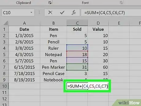
1Use the SUM function to add two or more cells. Select the cell you want the summation to output to. Then, type an equals sign (=), SUM, and the cells you’re summing enclosed in parenthesis. The function should look like this: =SUM(your numbers here).
- For example, =SUM(C4,C5,C6,C7) will add the numbers contained in the 4 cells within the parentheses.
-
2Use the SUM function to add a range of cells. If you provide a starting and ending cell, separated by a colon (:), you can sum large sections of the spreadsheet. The function should look like this: =SUM(cell1:cell2)' where “cell1” and “cell2” are your starting and ending cell respectively.
- For example, =SUM(C4:C7) sums the values in C4 to C7.
- You don't have to type out “C4:C7”. After typing “=SUM(” you can select a range by clicking and dragging your cursor from cell C4 to C7. The range will appear in the formula following the open parenthesis. Add the closing parenthesis at the end, and you're done!
- For a large range of numbers, this is much faster than clicking on each cell individually.
-
3Use the AutoSum Wizard. If you’re using Excel 2007 or later, an alternative to typing “=SUM” is using AutoSum.[1]
- Select the cell you want the summation to output to.
- Go to the Format tab > AutoSum drop-down arrow > Sum.
- Select the range of cells you want to sum.
- AutoSum might be limited to contiguous cell ranges in some versions of Excel; if you want to skip cells in your calculation, it may not work correctly.
-
4Copy/paste data into other cells. Since the cell with the function holds both the sum value and the sum function, you have to consider which you want copied.
- Copy the cell with the summation by pressing Ctrl + c (Windows) or Cmd + c (Mac). Then, select another cell and go to the Home tab > Clipboard drop-down and select either Paste Formulas or Paste Values.
-
5Reference sums in other functions. You can use the value of your summation cell in other functions. Rather than making a new summation or typing out the number value of your previous function, you can reference the original sum cell in other calculations.
- For example, let’s say you create a summation function for column C in C20 and column D in D20. You can add these sums by selecting a new cell and typing “=SUM(C20, D20)”
- This essentially nests your two summations into a third summation formula. Then, if your summation of C or D changes, this third summation will automatically update.
Using the SUMIF Function
-
1Use the basic SUMIF function. The SUMIF function allows you to sum values when they meet a criteria. The criteria can be within the range of values itself, or in a different range that is the same size as the values range. If the criteria is in the range itself, follow these steps:[2]
- Type =SUMIF( in a new cell.
- Select or type the range of cells you want to sum, then type a comma (,).
- Type a numerical criteria in double quotation marks, then type a closing parenthesis.
- For example, if you want to only sum numbers in a range that are greater than 10, you could type “=SUM(C1:C10, “>10”)”
-
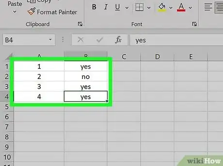
2Set up your data for SUMIF. If you’re using the optional parameter [sum_range], you’ll need separate columns for the range you want compared to the criteria and the range you want to sum. There are multiple ways to format a spreadsheet, but here’s a basic setup for SUMIF:
- Create one column with number values and a second column with a conditional value, like “yes” and “no”.
- For example, a column with 4 rows with values 1, 2, 3, and 4 and a second column with values of “yes” or “no”.
- This setup is similar to using VLOOKUP.
-
3Enter the function into a cell. To create a SUMIF formula using the optional [sum_range], follow these steps:
- Select a new cell and enter “=SUMIF(”
- range — Select or type a range of values to compare to the criteria. Then type a comma (,). This will be the range in the column where you placed your conditional values.
- criteria — Type in the criteria. This can be numerical, text-based, or boolean (TRUE/FALSE). Enclose this criteria with double-quotation marks. Then type a comma (,).
- sum_range — Select or type a range of values to sum. This will be the column you created with number values.
- The sum_range argument should be the same shape and size as range. The SUMIF formula will check the value in each range cell and add the respective sum_range cell to the sum.
- For example: “=SUMIF(C1:C4, “yes”, B1:B4)” will sum values in the range B1:B4 if the cell in C1:C4 is the string “yes”.
Using the SUMIFS Function
-
1Setup your data table. The setup is similar to SUMIF, but can support multiple criteria with multiple ranges.[3]
- Create one column with number values. These are the values you’ll sum if the criteria in the criteria ranges are met.
- Create multiple columns containing conditional values (e.g. yes/no, TRUE/FALSE, locations, dates, numeric values).
-
2Enter your SUMIFS function. To create a SUMIFS formula using multiple criteria, follow these steps:
- Select a new cell and enter “=SUMIFS(”
- sum_range — Select or type a range of cells to sum. Then type a comma (,). This will be the range in the column where you typed your number values.
- criteria_range1 — Select or type a range of values to compare to criteria1. Then type a comma (,). This will be one range in a column where you placed conditional values.
- criteria1 — Type in a criteria. This can be numerical, text-based, or boolean (TRUE/FALSE). Enclose this criteria with double-quotation marks. Then type a comma (,).
- criteria_range2 — Select or type a range of values to compare to criteria2. Then type a comma (,). This will be the second range in a column where you placed conditional values.
- criteria2 — Type in a criteria. This can be numerical, text-based, or boolean (TRUE/FALSE). Enclose this criteria with double-quotation marks. Then type a comma (,).
- Continue creating additional criteria_range and criteria as needed.
- The sum_range argument should be the same shape and size as every criteria_range. The SUMIFS formula will check the value in each criteria_range cell and add the respective sum_range cell to the sum.
- For example: “=SUMIFS(B1:B4, C1:C4, “yes”, D1:D4, “california”)” will sum values in the range B1:B4 if the cell in C1:C4 is the string “yes” and the cell in D1:D4 is the string “california”.
Community Q&A
-
QuestionNeed help adding results of very long formulas. The SUM works only if written in one single very long line.
 Community AnswerYou can establish ranges for SUM using a colon (:). This means you can skip all of the cells in between instead of adding them together one by one.
 -
QuestionWhat does the number one mean in =$J$1* - E4?
 Community AnswerThe $ both in front of the J and 1 mean that its reference is 'locked'. That means if you copy and paste the formula, or use the Excel Fill Handle (the little click-and-drag bit on the bottom-right of a cell when you click on it), the parts that immediately follow the $ stay the exact same. For instance, if it were just $J1, instead of $J$1, copying and pasting it a 4 rows down, the cell reference would be $J4; if it were J$1, copying and pasting it to the left one column would make the cell reference I$1.
References
- ↑ https://support.microsoft.com/en-us/office/use-autosum-to-sum-numbers-543941e7-e783-44ef-8317-7d1bb85fe706
- ↑ https://support.microsoft.com/en-us/office/sumif-function-169b8c99-c05c-4483-a712-1697a653039b
- ↑ https://support.microsoft.com/en-us/office/sumifs-function-c9e748f5-7ea7-455d-9406-611cebce642b
About This Article
1. Use the SUM function for ranges with numeric data.
2. Use the plus sign for small, quick sums.
3. Use the SUMIF function to specify a condition.
4. Use the SUMIFS function for complex logical statements.

