How to Show Hidden Columns in Microsoft Excel: Quick Guide

Quickly display one or more hidden columns in your Excel spreadsheet

Written by Kyle Smith

Last Updated: February 25, 2023

Using the Column Drag Tool

|

Using Right Click

|

Unhiding One Column with the Name Box

|

Unhiding All Columns

|

Q&A

|

Tips

Are you having trouble viewing certain columns in your Excel workbook? This wikiHow guide shows you how to display a hidden column in Microsoft Excel. You can do this on both the Windows and Mac versions of Excel. There are multiple simple methods to unhide hidden columns. You can drag the columns, use the right-click menu, or format the columns.

Things You Should Know

Hover your cursor to the right of the hidden columns, then click and drag to the right to unhide them.
Alternatively, select the columns adjacent to the hidden columns. Then right-click and select Unhide.
You can also go to Home > Format > Hide & Unhide to show hidden columns.

Method 1

Method 1 of 4:

Using the Column Drag Tool

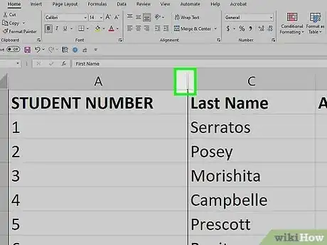
1
Hover your cursor directly to the right of the hidden columns. When your cursor is between the column letters adjacent to the hidden columns, the cursor will change into two parallel lines with two arrows pointing horizontally.
- You can identify hidden columns by looking for two lines between column letters.
- Your cursor needs to be to the right of the two lines for this method. Placing the cursor to the left will increase the column size of the left adjacent column.
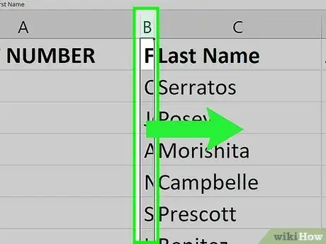
2
Click and drag to the right. This will unhide the hidden columns between the adjacent columns.
- Alternatively, you can double-click to immediately unhide the hidden column.
Advertisement
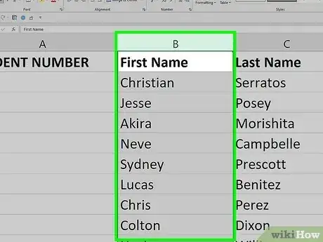
3
Release the mouse button. This will confirm the size of the unhidden columns. You’re ready to move some columns, sort your data, and add up column values!

Method 2

Method 2 of 4:

Using Right Click

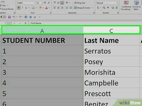
1
Select the columns on both sides of the hidden columns. To do this:
- Hold down the ⇧ Shift key while you click both letters above the column
- Click the left column next to the hidden columns.
- Click the right column next to the hidden columns.
- The columns will be highlighted when you successfully select them.
- For example, if column B is hidden, you should click A and then C while holding down ⇧ Shift.
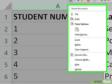
2
Right-click either of the selected columns. This will open the right-click pop up menu.
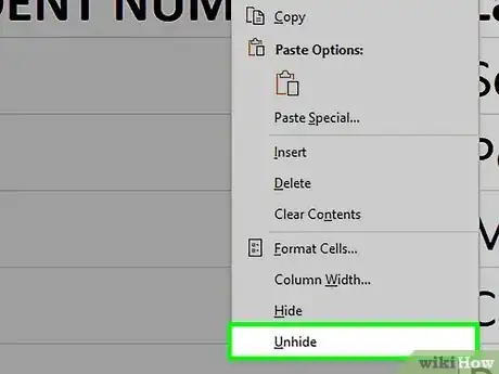
3
Select Unhide in the right-click menu. The hidden columns between the two selected columns will be unhidden.
- For more helpful excel tricks, check out our intro guide to Excel.

Method 3

Method 3 of 4:

Unhiding One Column with the Name Box

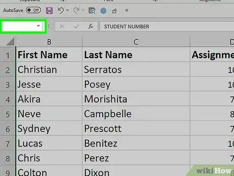
1
Click the Name Box. This is the drop down box to the left of the formula box.^{[1]
X
Trustworthy Source
Microsoft Support
Technical support and product information from Microsoft.
Go to source}
- This method is great for unhiding the first column (A) since there isn't a column to its left that you can select to access the right-click Unhide menu option.
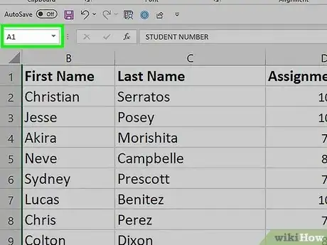
2
Type A1 in the Name Box and press ↵ Enter. Replace A with the letter of the column you want to unhide.
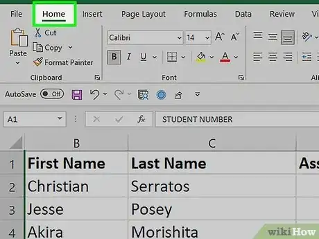
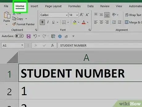
3
Click the Home tab. It's in the upper-left corner of the Excel window.
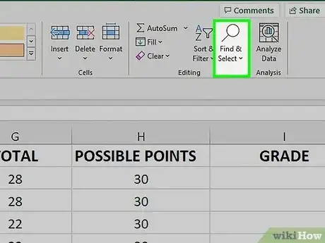
4
Click Find & Select. This is in the "Editing" group in the Home tab. A drop down menu will open.
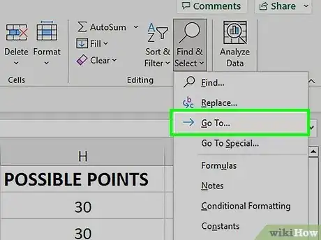
5
Select Go To. This will open the "Go To" window.
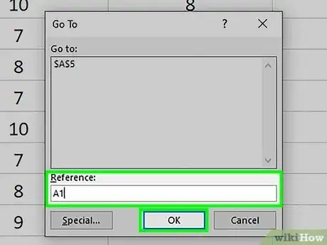
6
Type A1 in the "Reference" box and click OK.
7
Click the Home tab. It's in the upper-left corner of the Excel window.
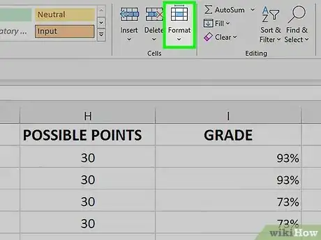
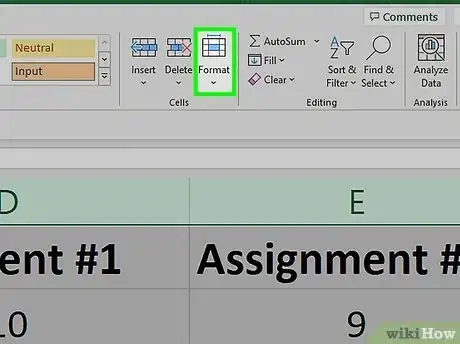
8
Click Format. This button is in the "Cells" section of the Home tab; you'll find this section on the right side of the toolbar. A drop down menu will appear.^{[2]
X
Research source}
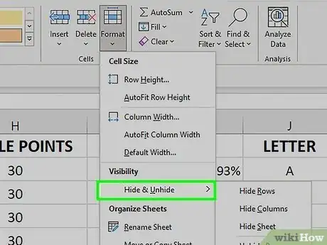
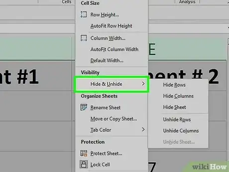
9
Select Hide & Unhide. This option is below the "Visibility" heading in the Format drop down menu. Selecting it will open a pop up menu.
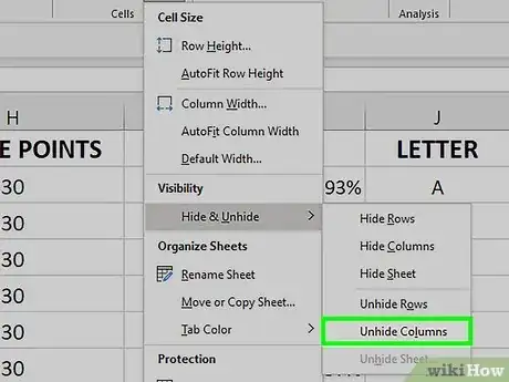
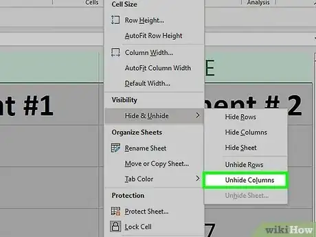
10
Click Unhide Columns. It's near the bottom of the Hide & Unhide menu. Doing so will immediately unhide the column you selected in the Name Box.

Method 4

Method 4 of 4:

Unhiding All Columns

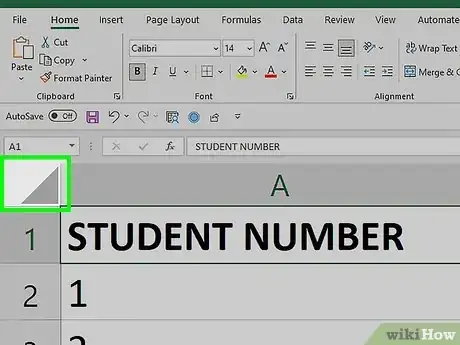
1
Click the triangle in the top left corner of the spreadsheet. This is next to the row 1 label and column A label. Clicking the triangle will select the entire spreadsheet.
- Hiding columns can be useful for when you have data you don’t need at the moment, but want to keep in the spreadsheet. For example, if you’re tracking your bills in Excel, you might want to hide purchase categories when you’re only working with the sum totals.
2
Click the Home tab. It's in the upper-left corner of the Excel window.
3
Click Format. This button is in the "Cells" section of the Home tab; you'll find this section on the right side of the toolbar. A drop down menu will appear.
4
Select Hide & Unhide. This option is below the "Visibility" heading in the Format drop down menu. Selecting it will open a pop up menu.
5
Click Unhide Columns. It's near the bottom of the Hide & Unhide menu. Doing so will immediately unhide every hidden column in the sheet.

Community Q&A

Question

What do I do if the hidden columns are A and B?

Community Answer

You can select the whole document and do the steps above to retrieve all hidden columns.
Question

What do I do if I've followed the instructions provided, but I still cannot unhide column A in Excel?

Community Answer

Try unfreezing the column and unhiding, or freezing then unfreezing then unhiding. This process will work.
Question

If column A is hidden in excel, how do I find it?

Community Answer

Just use the search bar on top and type there "A1" the hidden column should appear.