How to Sort Microsoft Excel Columns Alphabetically

Last Updated: December 16, 2022 Approved

Sorting your data alphabetically can help you organize directories, email lists, and lists of clients. This wikiHow article will teach you how to sort Microsoft Excel data alphabetically.

Method 1

Method 1 of 2:

Sorting Alphabetically

Download Audio

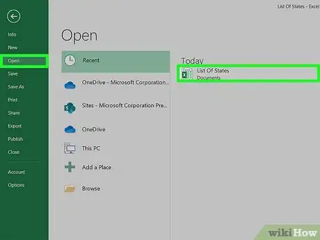
1
Open your project in Microsoft Excel. You can do this by going to File > Open within Excel or you can right-click the project file and select Open with > Excel.
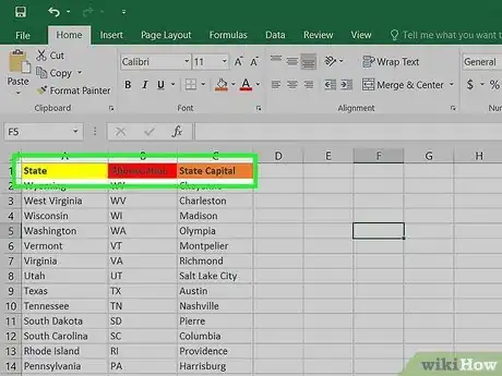
2
Format the header row. The header row is the top row of your spreadsheet, with the names of your columns. Excel will sometimes sort this row thinking it is part of your data, especially if your spreadsheet is entirely text. Here are a few ways to prevent this:
- Format your header row differently. For example, bold the text or make it a different color.^{[1]
  X
  Research source}
- Make sure there are no blank cells in your header row.^{[2]
  X
  Research source}
- If Excel still sorts the headers, select the header row and use the top ribbon menu to click Home > Editing > Sort & Filter > Custom Sort > My data has headers.^{[3]
  X
  Research source}
Advertisement
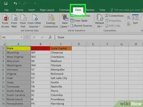
3
Select the column you wish to alphabetize. You can click the header cell for that column, or the letter above it (A, B, C, D, etc.).
- Press and hold Ctrl/Opt to select more than one column.
4
Click the Data tab. Click Data in the top menu to view Data options in the ribbon menu above your spreadsheet.
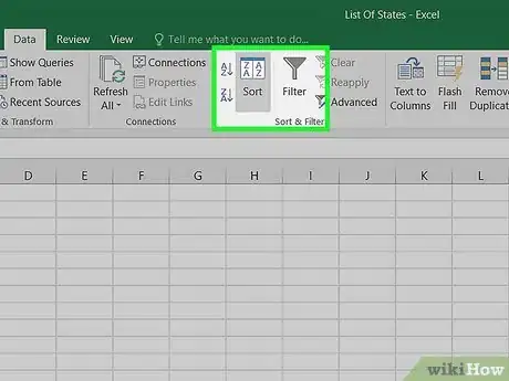
5
Look for the Sort and Filter section. The ribbon menu is divided into related areas, with the name under each one. Look for the area labeled Sort & Filter.
- If you don't see it on the Data menu, try returning to the Home tab and looking for a Sort & Filter button in the Editing section.
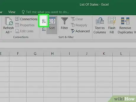
6
Click the A → Z button. To sort the spreadsheet in alphabetical order, just click the A → Z symbol in the Sort and Filter section. This will rearrange the spreadsheet in alphabetical order of the selected column. On most versions of Excel, this button is in the top left corner of the Sort and Filter section.
- To sort it in reverse alphabetical order instead, click the Z → A symbol instead.

Method 2

Method 2 of 2:

Sorting by Last Name

Download Audio

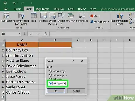
1
Insert a new blank column. Place this immediately to the right of the names column.
- Use this when your spreadsheet uses full names in a single cell. If you have full names listed in a single column, alphabetizing will only sort by the first name. With these instructions, you can divide the names into two columns first so you can sort by the last name column instead.^{[4]
  X
  Research source}
- To insert a blank column, select the letter row to the left of where you want the blank row to go (so if you want a new blank column to the right of A), select the first cell, then right-click it, and click Add Column to Right.
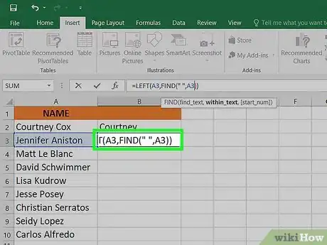
2
Enter the formula for first names. Enter this formula in the top cell of the new column: =LEFT(A1,FIND(" ",A1)) making sure to include the space between the quotation marks. This formula will look in the full name column and copy everything before the space.
- If necessary, replace both instances of A with the letter of the column that has the full names listed.
- Replace both instances of 1 with the number of the row you are typing in.
3
Copy this formula to the entire column. Click the header of this new column and copy-paste the formula you just entered. You should see all the first names appear on their own in this column.
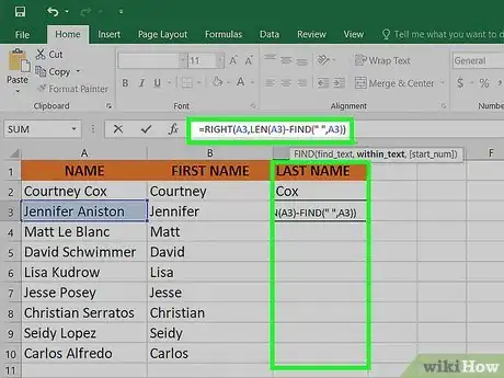
4
Create the last name column. Create a new column to the right of the first name column and enter this formula: =RIGHT(A1,LEN(A1)-FIND(" ",A1)). Copy-paste this formula to populate the column with last names.
5
Sort by the last name column. You may now sort the last name column alphabetically, as described in the Sorting Alphabetically method.

Community Q&A

Question

What is the shortcut key for merging cells?

Community Answer

Hold the key until an overlay appears on the ribbon. Press to select the Home tab. Press to select Merge and Center. Then, press to merge and center the selected cells.
Question

Is there a maximum number of lines in Excel?

Community Answer

In Excel 2010, the maximum worksheet size is 1,048,576 rows by 16,384, so I don't think so.