How to Round in Microsoft Excel: ROUND, Formatting, and More

Round a number to the decimal place you want in Excel

Written by Kyle Smith

Last Updated: February 27, 2023 Tested

The ROUND Function

|

Other Rounding Functions

|

Increase/Decrease Decimal Buttons

|

Cell Formatting

|

Q&A

This wikiHow guide shows you how to round the value of a cell using the ROUND formula, and how to use cell formatting to display cell values as rounded numbers. Both methods are easy to set up and use! There are also a few other helpful functions (ROUNDUP, ROUNDDOWN, MROUND, EVEN, ODD) for rounding numbers in different ways.

Things You Should Know

Use the function ROUND(number, num_digits) to round a number to the nearest number of digits specified.
Use other functions like ROUNDUP and ROUNDDOWN to change the rounding method.
Use cell formatting to display numbers as rounded while maintaining the original value.

Section 1 of 4:

The ROUND Function

1
Enter the data into your spreadsheet. Rounding numbers has plenty of useful applications! For example, if you’re tracking your bills in Excel, you can round the values to integer numbers to see a simpler view of your purchases.
2
Click a cell next to the one you want to round. This allows you to enter a formula into the cell.

Advertisement
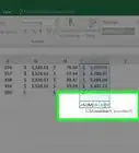
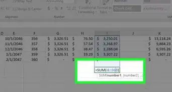
3
Type =ROUND into the “fx” field. The field is at the top of the spreadsheet. The equal sign indicates that you’re creating a formula rather than typing text.
4
Type an open parenthesis after “ROUND.” The content of the “fx” box should now look like this: =ROUND(.
5
Click the cell that you want to round. This inserts the cell's location (e.g., A1) into the formula. If you clicked A1, the “fx” box should now look like this: =ROUND(A1.
6
Type a comma followed by the number of digits to round to. For example, if you wanted to round the value of A1 to 2 decimal places, your formula would so far look like this: =ROUND(A1,2.
- Use 0 as the decimal place to round to the nearest whole number.
- Use a negative number to round by multiples of 10. For example, =ROUND(A1,-1will round the number to the next multiple of 10.
7
Type a closed parenthesis to finish the formula. The final formula should look like this, using the example of rounding A1 to 2 decimal places: =ROUND(A1,2).
8
Press ↵ Enter or ⏎ Return. This runs the ROUND formula and displays the rounded value in the selected cell. Now you’re ready to SUM some numbers or create a chart.
- You can copy this formula as needed to round other numbers to the same specification.

Section 2 of 4:

Other Rounding Functions

1
Use ROUNDUP to round a number up. The ROUNDUP function uses the same parameters as the ROUND function, so you can round up to a specified number of digits. For example, =ROUNDUP(A1, 2) would round up the number in A1 to the nearest hundredths place.
- If A1 were 10.732, it would round up to 10.74.
2
Use ROUNDUP to round a number down. The ROUNDDOWN function uses the same parameters as the ROUND function, so you can round down to a specified number of digits. For example, =ROUNDDOWN(A1, 2) would round down the number in A1 to the nearest hundredths place.
- If A1 were 10.732, it would round up to 10.73.
3
Use MROUND to round a number to a nearest multiple. The MROUND function allows you to input a specific multiple that you want to round to. For example, =MROUND(A1, 15) would round the number in A1 to the nearest multiple of 15.
- If A1 were 10.732, it would round to 15.
4
Use EVEN to round up a number to the nearest even integer. The EVEN function only has one argument, the number you’re rounding. For example, =EVEN(A1) would round the number in A1 up to the nearest even integer.
- If A1 were 10.732, it would round to 12.
5
Use ODD to round up a number to the nearest even integer. The ODD function only has one argument, the number you’re rounding. For example, =ODD(A1) would round the number in A1 up to the nearest odd integer.
- If A1 were 10.732, it would round to 11.

Section 3 of 4:

Increase/Decrease Decimal Buttons

1
Enter the data into your spreadsheet. After making a spreadsheet in Excel, getting the formatting right requires knowing the formatting tools.
- Note that this method doesn’t change the actual value in the cell, only how it appears in the spreadsheet.
2
Highlight any cell(s) you want rounded. To highlight multiple cells, click the top left-most cell of the data, then drag your cursor down and to the right until all cells are highlighted.
3
Click the Decrease Decimal button to show fewer decimal places. It's the button that says .00 → .0 on the Home tab on the “Number” panel (the last button on that panel).
- Example: Clicking the Decrease Decimal button would change $4.36 to $4.4.
4
Click the Increase Decimal button to show more decimal places. This gives a more precise value (rather than rounding). It's the button that says ←.0 .00 (also on the “Number” panel).
- Example: Clicking the Increase Decimal button might change $2.83 to $2.834.

Section 4 of 4:

Cell Formatting

1
Enter your data series into your Excel spreadsheet.
- Note that this method doesn’t change the actual value in the cell, only how it appears in the spreadsheet.
2
Highlight any cell(s) you want rounded. To highlight multiple cells, click the top left-most cell of the data, then drag your cursor down and to the right until all cells are highlighted.
3
Right-click any highlighted cell. A menu will appear.
4
Click Number Format or Format Cells. The name of this option varies by version.
5
Click the Number tab. It's either on the top or side of the window that popped up.
6
Click Number from the category list. It's on the side of the window.
7
Select the number of decimal places you want to round to. Click the down-arrow next to “Decimal places” to reduce the number of decimal places and round the numbers down.
- Example: To round 16.47334 to 1 decimal place, select 1 from the menu. This would cause the value to be rounded to 16.5.
- Example: To round the number 846.19 to a whole number, select 0 from the menu. This would cause the value to be rounded to 846.
8
Click OK. It's at the bottom of the window. The selected cells are now rounded to the selected decimal place.
- To apply this setting to all values on the sheet (including those you add in the future):
  - Click anywhere on the sheet to remove the highlighting.
  - Click the Home tab at the top of Excel.
  - Click the drop-down menu on the “Number” panel.
  - Select More Number Formats.
  - Set the desired “Decimal places” value, then click OK to make it the default for the file.
  - In some versions of Excel, you'll have to click the Format menu, then Cells, followed by the Number tab to find the “Decimal places” menu.

Community Q&A

Question

How do you round to 2 decimal places in Excel?

wikiHow Staff Editor
Staff Answer
This answer was written by one of our trained team of researchers who validated it for accuracy and comprehensiveness.

wikiHow Staff Editor

Staff Answer

Go to the “Math & Trig” menu in the “Formulas” tab. Select “ROUND” from the drop-down menu. In the “Number” field, enter the number you want to the round or the ID of the cell containing the number. In the “Num_Digits” field, enter the positive integer “2” to indicate that you want 2 digits to appear after the decimal point.
Question

How do you round to the nearest whole number in Excel?

wikiHow Staff Editor
Staff Answer
This answer was written by one of our trained team of researchers who validated it for accuracy and comprehensiveness.

wikiHow Staff Editor

Staff Answer

When you use the “ROUND” function, enter a -1 in the “Num_Digits” field. This indicates that you want the rounding to happen just to the left of the decimal point, so you will round to a whole number instead of a decimal.
Question

How do you show 2 decimal places in Excel without rounding?

wikiHow Staff Editor
Staff Answer
This answer was written by one of our trained team of researchers who validated it for accuracy and comprehensiveness.

wikiHow Staff Editor

Staff Answer

To do this, you can use the TRUNC (“Truncate”) function. Write the formula =TRUNK, followed by 2 numbers in parentheses. The first is the number you want to truncate, the second is the decimal place you’d like to display. So, for instance, =TRUNC(27.3476,2) would give you 27.34, with no rounding.