This article was co-authored by wikiHow staff writer, Nicole Levine, MFA. Nicole Levine is a Technology Writer and Editor for wikiHow. She has more than 20 years of experience creating technical documentation and leading support teams at major web hosting and software companies. Nicole also holds an MFA in Creative Writing from Portland State University and teaches composition, fiction-writing, and zine-making at various institutions.
This article has been viewed 201,779 times.
Learn more...
If you’ve ever tried printing a large Microsoft Excel worksheet, you’ve undoubtedly encountered some awkward-looking print jobs. Excel’s automatic page breaks don’t exactly take your custom data views into consideration. In order to control exactly which rows and columns appear on your printed pages, you’ll need to insert manual page breaks. Fortunately, this is simple and easy to visualize in Excel’s Page Break view.
Steps
Getting Excel Ready
-
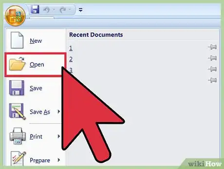
1Open your spreadsheet. Click “File,” then “Open,” and navigate to the folder that contains your spreadsheet. Double-click the file name to view it in Excel.
-
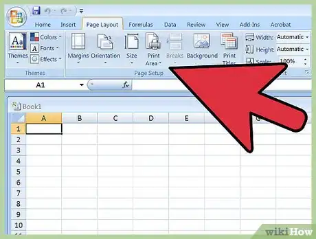
2Open the Page Setup options.[1] Click the “Page Layout” tab at the top of the screen and locate the group called “Page Setup.” To view the options, click the small arrow at the bottom right of the Page Setup group.Advertisement
-
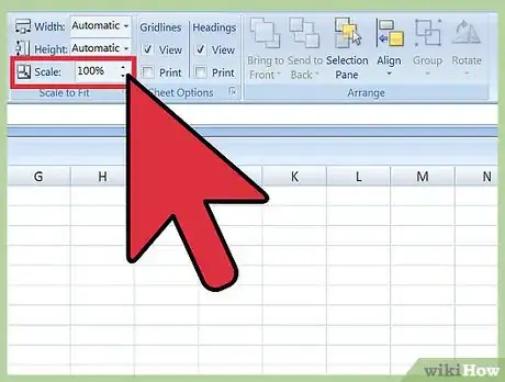
3Enable adjusted scaling. On the “Page” tab of the Page Setup options, locate the section called “Scaling.” Select “Adjust to:” and change the percentage to
100%. Click “OK” to save this setting. -
4Enter Page Break view. This view allows you to see where automatic page breaks occur (indicated by blue dotted lines). Knowing where the automatic page breaks occur will help you place your new page breaks appropriately. Click the “View” tab and select “Page Break Preview” from the Workbook Views group to launch this view.
Inserting and Managing Breaks
-
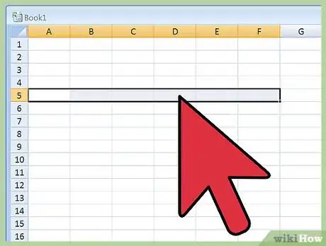
1Click the row below your desired horizontal page break location.[2] For example, if you want to place a horizontal page break between rows 4 and 5, select row 5.
-
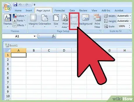
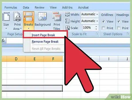
2Insert the horizontal page break. Return to the “Page Layout” tab and click the arrow beneath the “Breaks” icon. From the options, select “Insert Page Break.” A thick line will appear where the manual break was inserted.
-
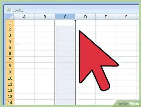
3Select the column to the right of your desired vertical line break. If you want to insert a vertical line break between columns C and D, for example, select column D.
-
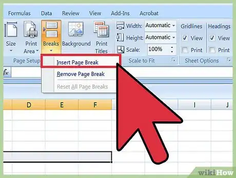
4Insert the vertical page break. On the “Page Layout” tab, click the arrow beneath the “Breaks” icon, then select “Insert Page Break.” A thick vertical line will indicate the location of your new break.
-
5Move your page break. If you decide your page break should occur at a different location than where you’ve originally inserted it, hold your mouse over the break until an arrow appears, then drag the arrow to another location.
-
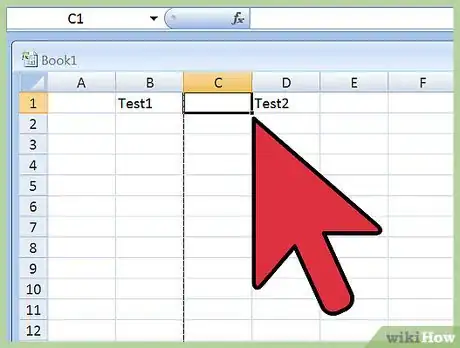
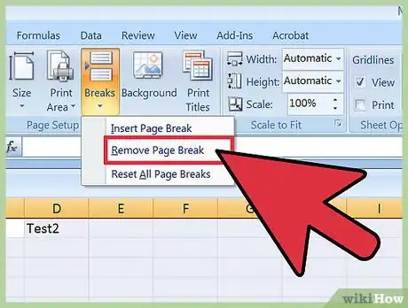
6Delete a page break. If you decide you no longer want a page break you’ve inserted, it’s possible to delete the break.
- Delete a vertical break: Select the column directly to the right of your vertical page break. Click the arrow beneath the “Breaks” icon and select “Remove Page Break.”
- Delete a horizontal line break: Select the column just below the horizontal page break, then click the arrow beneath the “Breaks” icon. Select “Remove Page Break.”
-
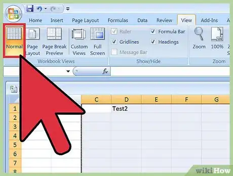
7Return to Normal view. If you don’t want to see the page breaks while you work, click the “View” menu at the top of the screen, then select “Normal.” You can switch between these two views as needed.
