How to Assess Statistical Significance

Co-authored by Bess Ruff, MA

Last Updated: February 6, 2023 References

Hypothesis testing is guided by statistical analysis. Statistical significance is calculated using a p-value, which tells you the probability of your result being observed, given that a certain statement (the null hypothesis) is true.^{[1]
X
Trustworthy Source
PubMed Central
Journal archive from the U.S. National Institutes of Health
Go to source} If this p-value is less than the significance level set (usually 0.05), the experimenter can assume that the null hypothesis is false and accept the alternative hypothesis. Using a simple t-test, you can calculate a p-value and determine significance between two different groups of a dataset.

Part 1

Part 1 of 3:

Setting up Your Experiment

1
Define your hypotheses. The first step in assessing statistical significance is defining the question you want to answer and stating your hypothesis. The hypothesis is a statement about your experimental data and the differences that may be occurring in the population. For any experiment, there is both a null and an alternative hypothesis.^{[2]
X
Research source} Generally, you will be comparing two groups to see if they are the same or different.
- The null hypothesis (H₀) generally states that there is no difference between your two data sets. For example: Students who read the material before class do not get better final grades.
- The alternative hypothesis (H_a) is the opposite of the null hypothesis and is the statement you are trying to support with your experimental data. For example: Students who read the material before class do get better final grades.
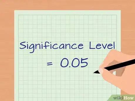
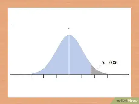
2
Set the significance level to determine how unusual your data must be before it can be considered significant. The significance level (also called alpha) is the threshold that you set to determine significance. If your p-value is less than or equal to the set significance level, the data is considered statistically significant.^{[3]
X
Trustworthy Source
Simply Psychology
Popular site for evidence-based psychology information
Go to source}
- As a general rule, the significance level (or alpha) is commonly set to 0.05, meaning that the probability of observing the differences seen in your data by chance is just 5%.
- A higher confidence level (and, thus, a lower p-value) means the results are more significant.
- If you want higher confidence in your data, set the p-value lower to 0.01. Lower p-values are generally used in manufacturing when detecting flaws in products. It is very important to have high confidence that every part will work exactly as it is supposed to.
- For most hypothesis-driven experiments, a significance level of 0.05 is acceptable.
Advertisement
3
Decide to use a one-tailed or two-tailed test. One of the assumptions a t-test makes is that your data is distributed normally. A normal distribution of data forms a bell curve with the majority of the samples falling in the middle. The t-test is a mathematical test to see if your data falls outside of the normal distribution, either above or below, in the “tails” of the curve.^{[4]
X
Research source}
- A one-tailed test is more powerful than a two-tailed test, as it examines the potential of a relationship in a single direction (such as above the control group), while a two-tailed test examines the potential of a relationship in both directions (such as either above or below the control group).^{[5]
  X
  Research source}
- If you are not sure if your data will be above or below the control group, use a two-tailed test. This allows you to test for significance in either direction.
- If you know which direction you are expecting your data to trend towards, use a one-tailed test. In the given example, you expect the student’s grades to improve; therefore, you will use a one-tailed test.
4
Determine sample size with a power analysis. The power of a test is the probability of observing the expected result, given a specific sample size. The common threshold for power (or β) is 80%. A power analysis can be a bit tricky without some preliminary data, as you need some information about your expected means between each group and their standard deviations. Use a power analysis calculator online to determine the optimal sample size for your data.^{[6]
X
Research source}
- Researchers usually do a small pilot study to inform their power analysis and determine the sample size needed for a larger, comprehensive study.
- If you do not have the means to do a complex pilot study, make some estimations about possible means based on reading the literature and studies that other individuals may have performed. This will give you a good place to start for sample size.

Part 2

Part 2 of 3:

Calculating the Standard Deviation

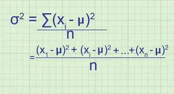
1
Define the formula for standard deviation. The standard deviation is a measure of how spread out your data is. It gives you information on how similar each data point is within your sample, which helps you determine if the data is significant. At first glance, the equation may seem a bit complicated, but these steps will walk you through the process of the calculation. The formula is s = √∑((x_i – µ)²/(N – 1)).^{[7]
X
Research source}
- s is the standard deviation.
- ∑ indicates that you will sum all of the sample values collected.
- x_i represents each individual value from your data.
- µ is the average (or mean) of your data for each group.
- N is the total sample number.
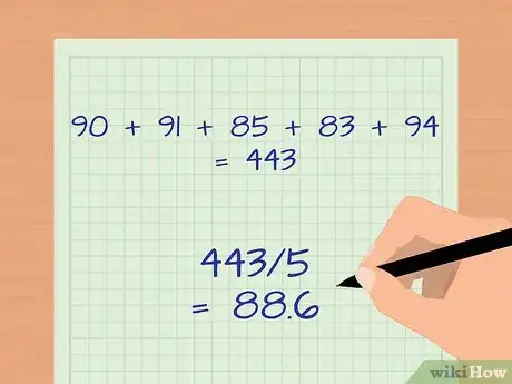
2
Average the samples in each group. To calculate the standard deviation, first you must take the average of the samples in the individual groups. The average is designated with the Greek letter mu or µ. To do this, simply add each sample together and then divide by the total number of samples.^{[8]
X
Research source}
- For example, to find the average grade of the group that read the material before class, let’s look at some data. For simplicity, we will use a dataset of 5 points: 90, 91, 85, 83, and 94.
- Add all the samples together: 90 + 91 + 85 + 83 + 94 = 443.
- Divide the sum by the sample number, N = 5: 443/5 = 88.6.
- The average grade for this group is 88.6.
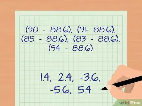
3
Subtract each sample from the average. The next part of the calculation involves the (x_i – µ) portion of the equation. You will subtract each sample from the average just calculated. For our example you will end up with five subtractions.^{[9]
X
Research source}
- (90 – 88.6), (91- 88.6), (85 – 88.6), (83 – 88.6), and (94 – 88.6).
- The calculated numbers are now 1.4, 2.4, -3.6, -5.6, and 5.4.
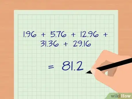
4
Square each of these numbers and add them together. Each of the new numbers you have just calculated will now be squared. This step will also take care of any negative signs. If you have a negative sign after this step or at the end of your calculation, you may have forgotten this step.^{[10]
X
Research source}
- In our example, we are now working with 1.96, 5.76, 12.96, 31.36, and 29.16.
- Summing these squares together yields: 1.96 + 5.76 + 12.96 + 31.36 + 29.16 = 81.2.
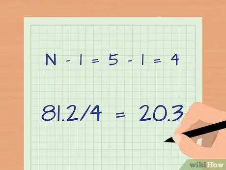
5
Divide by the total sample number minus 1. The formula divides by N – 1 because it is correcting for the fact that you haven’t counted an entire population; you are taking a sample of the population of all students to make an estimation.^{[11]
X
Research source}
- Subtract: N – 1 = 5 – 1 = 4
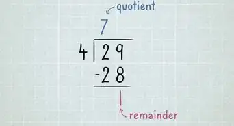
- Divide: 81.2/4 = 20.3
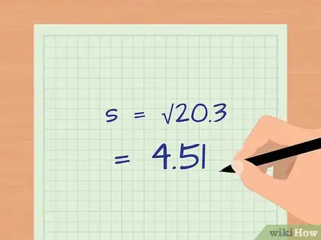
6
Take the square root. Once you have divided by the sample number minus one, take the square root of this final number. This is the last step in calculating the standard deviation. There are statistical programs that will do this calculation for you after inputting the raw data.^{[12]
X
Research source}
- For our example, the standard deviation of the final grades of students who read before class is: s =√20.3 = 4.51.

Part 3

Part 3 of 3:

Determining Significance

1
Calculate the variance between your 2 sample groups. Up to this point, the example has only dealt with 1 of the sample groups. If you are trying to compare 2 groups, you will obviously have data from both. Calculate the standard deviation of the second group of samples and use that to calculate the variance between the 2 experimental groups. The formula for variance is s_d = √((s₁/N₁) + (s₂/N₂)).^{[13]
X
Research source}
- s_d is the variance between your groups.
- s₁ is the standard deviation of group 1 and N₁ is the sample size of group 1.
- s₂ is the standard deviation of group 2 and N₂ is the sample size of group 2.
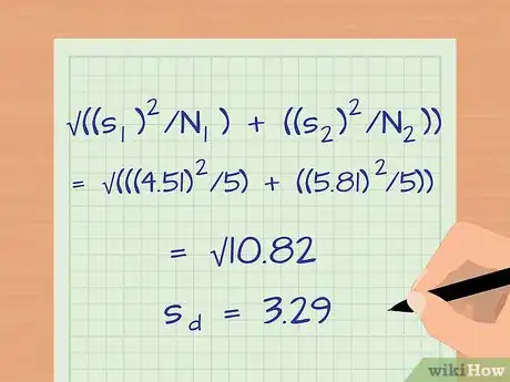
- For our example, let’s say the data from group 2 (students who didn’t read before class) had a sample size of 5 and a standard deviation of 5.81. The variance is:
  - s_d = √((s₁)²/N₁) + ((s₂)²/N₂))
  - s_d = √(((4.51)²/5) + ((5.81)²/5)) = √((20.34/5) + (33.76/5)) = √(4.07 + 6.75) = √10.82 = 3.29.
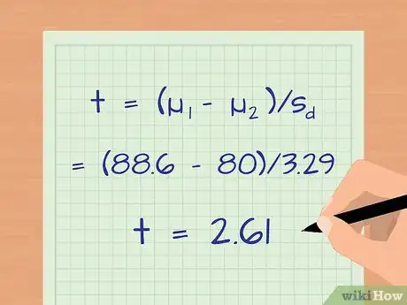
2
Calculate the t-score of your data. A t-score allows you to convert your data into a form that allows you to compare it to other data. T-scores allow you to perform a t-test that lets you calculate the probability of two groups being significantly different from each other. The formula for a t-score is: t = (µ₁ – µ₂)/s_d.^{[14]
X
Research source}
- µ₁ is the average of the first group.
- µ₂ is the average of the second group.
- s_d is the variance between your samples.
- Use the larger average as µ₁ so you will not have a negative t-value.
- For our example, let’s say the sample average for group 2 (those who didn’t read) was 80. The t-score is: t = (µ₁ – µ₂)/s_d = (88.6 – 80)/3.29 = 2.61.
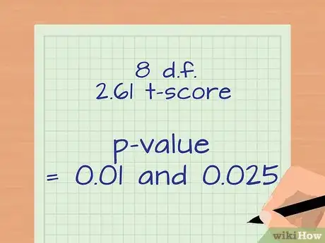
3
Determine the degrees of freedom of your sample. When using the t-score, the number of degrees of freedom is determined using the sample size. Add up the number of samples from each group and then subtract two. For our example, the degrees of freedom (d.f.) are 8 because there are five samples in the first group and five samples in the second group ((5 + 5) – 2 = 8).
4
Use a t table to evaluate significance. A table of t-scores^{[15]
X
Research source} and degrees of freedom can be found in a standard statistics book or online. Look at the row containing the degrees of freedom for your data and find the p-value that corresponds to your t-score.
- With 8 d.f. and a t-score of 2.61, the p-value for a one-tailed test falls between 0.01 and 0.025. Because we set our significance level less than or equal to 0.05, our data is statistically significant. With this data, we reject the null hypothesis and accept the alternative hypothesis:^{[16]
  X
  Research source} students who read the material before class get better final grades.
5
Consider a follow up study. Many researchers do a small pilot study with a few measurements to help them understand how to design a larger study. Doing another study, with more measurements, will help increase your confidence about your conclusion.
- A follow-up study can help you determine if any of your conclusions contained type I error (observing a difference when there isn’t one, or false rejection of the null hypothesis) or type II error (failure to observe a difference when there is one, or false acceptance of the null hypothesis).^{[17]
  X
  Research source}

Expert Q&A
Did you know you can get expert answers for this article? Unlock expert answers by supporting wikiHow

Question

What is the difference between ANOVA and t-test? I have categorical groups for weight and height and I want to compare the data in each group and see if there is significance.

Bess Ruff, MA
Environmental Scientist
Bess Ruff is a Geography PhD student at Florida State University. She received her MA in Environmental Science and Management from the University of California, Santa Barbara in 2016. She has conducted survey work for marine spatial planning projects in the Caribbean and provided research support as a graduate fellow for the Sustainable Fisheries Group.

Bess Ruff, MA

Environmental Scientist

Expert Answer

Support wikiHow by unlocking this expert answer.

A t-test is used to compare the means of ONLY 2 populations. If you want to compare the means of more than 2 populations, you will use an ANOVA.
Question

Can you explain degree of freedom, how you came to the number of P value range and how they are connected with the final steps?

Community Answer

The degrees of freedom is the number of samples in your population minus one. The minus one is from you using one degree of freedom to calculate the average.
Question

Why do you square your S1 in your example of variance, but not in your explanation of the formula?

Community Answer

The actual formula from the source he refers to for variance is the square root one. This leads me to believe that the notation without the square root is simply a mistake from the author.

Warnings

This analysis is specific to a t-test to test the differences between 2 normally distributed populations. You made need to use a different statistical test depending on the complexity of your dataset.

⧼thumbs_response⧽
Helpful 0 Not Helpful 0