This article was co-authored by wikiHow staff writer, Darlene Antonelli, MA. Darlene Antonelli is a Technology Writer and Editor for wikiHow. Darlene has experience teaching college courses, writing technology-related articles, and working hands-on in the technology field. She earned an MA in Writing from Rowan University in 2012 and wrote her thesis on online communities and the personalities curated in such communities.
This article has been viewed 48,736 times.
Learn more...
After you create a pivot table, you might need to edit it later. This wikiHow will show you how to edit a pivot table in Excel on your computer by adding or changing the source data. After you make any changes to the data for your Pivot Table, you will need to refresh it to see any changes.
Steps
-
1Open your project in Excel. To do this, double-click the Excel document that contains your pivot table in Finder (Macs) or File Explorer (Windows). Alternatively, if you already have Excel open, click File > Open and select the file that has your pivot table.
-
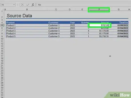
2Go to the spreadsheet page that contains the data for the pivot table. Click the tab that contains your data (e.g., Sheet 2) at the bottom of the Excel window.Advertisement
-
3Add or change your data. Enter the data that you want to add to your pivot table directly next to or below the current data.
- For example, if you have data in cells A1 through E10, you would add another column in the F column or another row in the 11 row.
- If you simply want to change the data in your pivot table, edit the data here. It won't be reflected in the pivot table until you refresh the data, though.
-
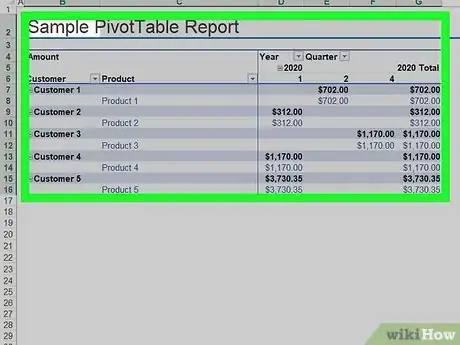
4Go back to the pivot table tab. Click the tab on which your pivot table is listed.
-
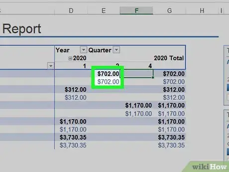
5Select your pivot table. Click the pivot table to select it.
-
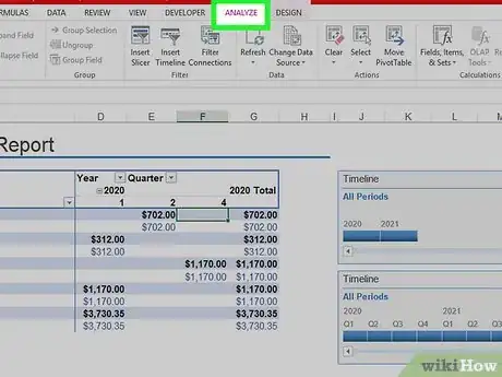
6Click the Analyze tab. It's in the middle of the editing ribbon that's at the top of the Excel window. Doing so will open a toolbar just below the editing ribbon.
- On a Mac, click the PivotTable Analyze tab here instead.
-
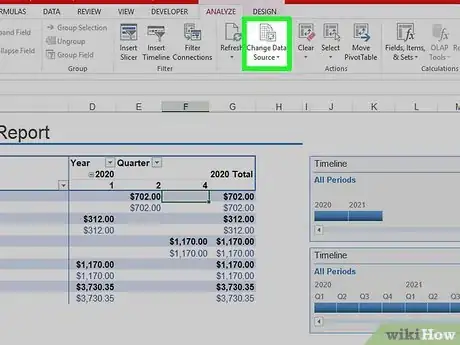
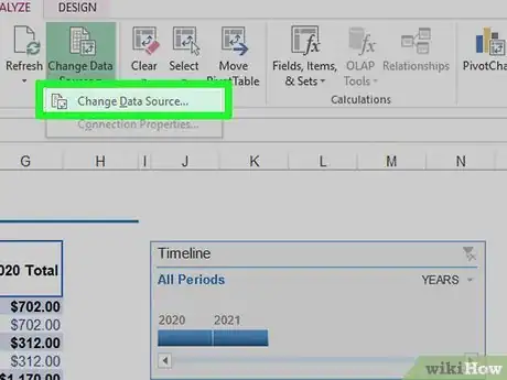
7Click Change Data Source. This option is in the "Data" section of the Analyze toolbar. A drop-down menu will appear.
-
8Click Change Data Source…. It's in the drop-down menu. Doing so opens a window.
-
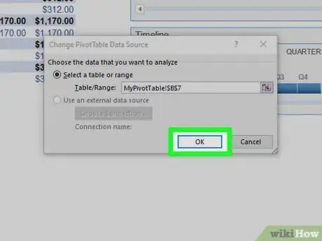
9Select your data. Click and drag from the top-left cell in your data group down to the bottom-left cell in the group. This will include the column(s) or row(s) that you added.
-
10Click OK. It's at the bottom of the window.
-
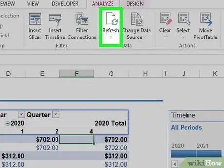
11Click Refresh. It's in the "Data" section of the toolbar.
- If you added a new column to your pivot table, check its box on the right side of the Excel window to display it.[1]
References
About This Article
1. Open your project in Excel.
2. Go to the spreadsheet that contains the data for the pivot table
3. Add or change your data.
4. Go back to the pivot table tab.
5. Select your pivot table.
6. Click Analyze tab (Windows) or PivotTable Analyze (Mac).
7. Click Change Data Source.
8. Click Change Data Source.
9. Select your data.
10. Click Ok.
11. Click Refresh.


