How to Create an Index in Excel

Last Updated: February 7, 2022

If your Excel workbook contains numerous worksheets, you can add a table of contents that indexes all of your sheets with clickable hyperlinks. This tutorial will teach you how to make an index of sheet names with page numbers in your Excel workbook without complicated VBA scripting, and how to add helpful "back to index" buttons to each sheet to improve navigation.

Part 1

Part 1 of 2:

Making the Index

1
Create an index sheet in your workbook. This sheet can be anywhere in your workbook, but you'll usually want to place the tab at the beginning like a traditional table of contents.
- To create a new sheet, click the + at the bottom of the active worksheet. Then, right-click the new tab, select Rename, and type a name for your sheet like Index or Worksheets.
- You can rearrange sheets by dragging their tabs left or right at the bottom of your workbook.
2
Type Page Number into cell A1 of your index sheet. Column A is where you'll be placing the page numbers for each sheet.

Advertisement
3
Type Sheet Name into cell B1 of your index sheet. This will be the column header above your list of worksheets.
4
Type Link into cell C1 of your index sheet. This is the column header that will appear above hyperlinks to each worksheet.
5
Click the Formulas tab. It's at the top of Excel.
6
Click Define Name. It's on the "Defined Names" tab at the top of Excel.
7
Type SheetList into the "Name" field. This names the formula you'll be using with the INDEX function.^{[1]
X
Research source}
8
Type the formula into the "Refers to" field and click OK. The formula is =REPLACE(GET.WORKBOOK(1),1,FIND("]",GET.WORKBOOK(1)),"").
9
Enter page numbers in column A. This is the only part you'll have to do manually. For example, if your workbook has 20 pages, you'll type 1 into A2, 2 into A3, etc., and continue numbering down until you've entered all 20 page numbers.
- To quickly populate the page numbers, type the first two page numbers into A2 and A3, click A3 to select it, and then drag the square at A3's bottom-right corner down until you've reached the number of pages in your workbook. Then, click the small icon with a + that appears at the bottom-right corner of the column and select Fill Series.
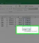
10
Type this formula into cell B2 of your index sheet. The formula is =INDEX(SheetList,A2). When you press Enter or Return, you'll see the name of the first sheet in your workbook.
11
Fill the rest of column B with the formula. To do this, just click B2 to select it, and then double-click the square at its bottom-right corner. This adds the name of each worksheet corresponding to the page numbers you typed into column A.
12
Type this formula into C2 of your worksheet. The formula is =HYPERLINK("#'"&B2&"'!A1","Go to Sheet"). When you press Enter or Return, you'll see a hyperlink to the first page in your index called "Go to Sheet."
13
Fill the rest of column C with the formula. To do this, click C2 to select it, and then double-click the square at its bottom-right corner. Now each sheet in your workbook has a clickable hyperlink that takes you right to that page.
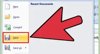
14
Save your workbook in the macro-enabled format. Because you created a named range, you'll need to save your workbook in this format.^{[2]
X
Trustworthy Source
Microsoft Support
Technical support and product information from Microsoft.
Go to source} Here's how:
- Go to File > Save.
- On the pop-up message that warns you about saving a macro-free workbook, click No.
- In the "Save as type" or file format menu, select Excel Macro-Enabled Workbook (*.xlsm) and click Save.

Part 2

Part 2 of 2:

Creating Hyperlinks Back to the Index

1
Click your index or table of contents sheet. If you have a lot of pages in your workbook, it'll be helpful to readers to add quick "Back to Index" or "Back to Table of Contents" links to each sheet so they don't have to scroll through lots of worksheet tabs after clicking to that page. Start by opening your index sheet.
2
Name the index. To do this, just click the field directly above cell A1, type Index, and then press Enter or Return.
- Don't worry if the field already contains a cell address.
3
Click any of the sheets in your workbook. Now you'll create your back button. Once you create a back button on one sheet, you can just copy and paste it onto other sheets.
4
Click the Insert tab. It's at the top of the screen.
5
Click the Illustrations menu and select Shapes. This option will be in the upper-left area of Excel.
6
Click a shape for your button. For example, if you want to create a back-arrow icon sort of like your web browser's back button, you can click the left-pointing arrow under the "Block Arrows" header.
7
Click the location where you want to place the button. Once you click, the shape will appear. If you want, you can change the color and look using the options at the top, and/or resize the shape by dragging any of its corners.
8
Type some text onto the shape. The text you type should be something like "Back to Index." You can double-click the shape to place the cursor and start typing right onto the actual shape
- You might need to drag the corner of the shape to resize it so the text fits.
- To place a text box on or near the shape before typing, just click the Shape Format menu at the top (while the shape is selected), click Text Box in the toolbar, and then click and drag a text box.
- You can stylize the text using the options in Text on the toolbar while the shape is selected.
9
Right-click the shape and select Link. This opens the Insert Hyperlink dialog.^{[3]
X
Trustworthy Source
Microsoft Support
Technical support and product information from Microsoft.
Go to source}
10
Click the Place in This Document icon. It's in the left panel.
11
Select your index under "Defined Names" and click OK. You might have to click the + next to the column header to see the Index option. This makes the text in the shape a clickable hyperlink that takes you right to the index.
12
Copy and paste the hyperlink to other sheets. To do this, just right-click the shape and select Copy. Then, you can paste it onto any other page by right-clicking the desired location and selecting the first icon under "Paste Options" (the one that says "Use Destination Theme" when you hover the mouse over it).