How to Remove Spaces Between Characters and Numbers in Excel

Written by Nicole Levine, MFA

Last Updated: August 18, 2022 Tested

Using Find and Replace

|

Using the Substitute Function

This wikiHow teaches you how to remove unwanted spaces from cells in an Excel spreadsheet.

Method 1

Method 1 of 2:

Using Find and Replace

1
Highlight the range in which you want to remove all spaces. For example, if you want to remove spaces from C2 through C30, highlight those cells.
2
Click the Edit menu.

Advertisement
3
Select Find.
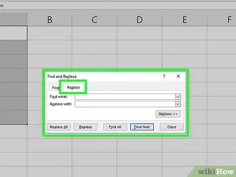
4
Select Replace…. A dialog box will appear.
5
Click the box beneath “Find What.”
6
Press the space bar on the keyboard. Make sure to press it only once.
7
Click Replace All. It’s the second button at the bottom of the window. The spaces are now removed from the selected cells. A pop-up will appear, letting you know how many spaces were removed.
8
Click OK.

Advertisement

Method 2

Method 2 of 2:

Using the Substitute Function

1
Click the top cell in a blank column. The cell must be on the same row as the first line of data in the column with the spaces.
- For example, if you want to remove spaces from column C, and C’s first row of data is in row 2 (C2), click the second cell in your blank column (e.g. E2, F2, G2, etc).
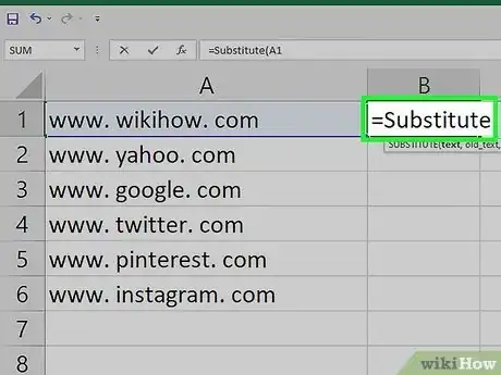
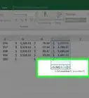
2
Type =Substitute.^{[1]
X
Research source}
3
Click the first cell in the column with spaces. For example, if you want to remove all of the spaces from the C column, click the first box (e.g. C2) in the column that isn’t the title.
- If you clicked cell C2, the formula should now look like this: =Substitute(C2 .
4
Type , (a comma). The cell should now look like this: =Substitute(C2,.
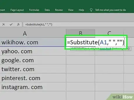
5
Type " ",. There’s a space between the two sets of quotes—this is important.
- The formula should now look like this: =Substitute(C2," ",.
6
Type ””). This time, there’s NO space between the sets of quotes.
- The formula should now look like this: =Substitute(C2,” “,””).
7
Press ↵ Enter or ⏎ Return. You will now see the contents of the selected cell (C2, in this example) without spaces in the new column.
- For example, if C2 said w ww . wikih ow .com, your new cell will say www.wikihow.com.
8
Click the cell with the formula you typed. The cell should now be highlighted.
9
Drag the fill handle down over the cells you want to fill. The data from each corresponding cell will now appear in your new column without spaces.
10
Copy the data from the new column to the original column. Your new space-free data is now in place.

Advertisement

You Might Also Like

Advertisement

References

↑ https://exceljet.net/excel-functions/excel-substitute-function

About This Article

Written by:

Nicole Levine, MFA

wikiHow Technology Writer

This article was co-authored by wikiHow staff writer, Nicole Levine, MFA. Nicole Levine is a Technology Writer and Editor for wikiHow. She has more than 20 years of experience creating technical documentation and leading support teams at major web hosting and software companies. Nicole also holds an MFA in Creative Writing from Portland State University and teaches composition, fiction-writing, and zine-making at various institutions. This article has been viewed 71,761 times.

How helpful is this?

Co-authors: 3

Updated: August 18, 2022

Views: 71,761

Categories: Microsoft Excel

Advertisement