This article was co-authored by Luigi Oppido and by wikiHow staff writer, Megaera Lorenz, PhD. Luigi Oppido is the Owner and Operator of Pleasure Point Computers in Santa Cruz, California. Luigi has over 25 years of experience in general computer repair, data recovery, virus removal, and upgrades. He is also the host of the Computer Man Show! broadcasted on KSQD covering central California for over two years.
This article has been viewed 3,745 times.
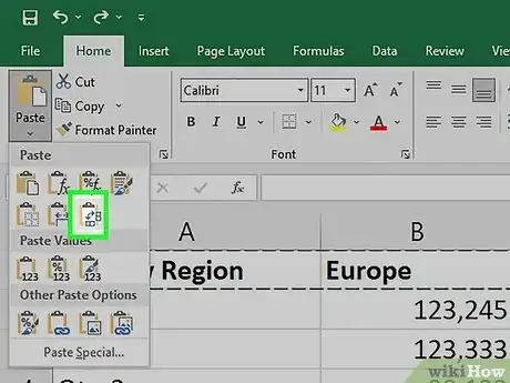
In Microsoft Excel, it can sometimes be useful to change the orientation of your data from rows to columns or vice versa. While there are a few different ways to do this, one quick and easy technique is to use paste transpose, which is a basic copy and paste operation. In this article, we’ll explain how to do it in just a few simple steps.
Steps
References
- ↑ https://support.microsoft.com/en-us/office/select-cell-contents-in-excel-23f64223-2b6b-453a-8688-248355f10fa9
- ↑ https://support.microsoft.com/en-us/office/transpose-rotate-data-from-rows-to-columns-or-vice-versa-3419f2e3-beab-4318-aae5-d0f862209744
- ↑ https://support.microsoft.com/en-us/office/transpose-rotate-data-from-rows-to-columns-or-vice-versa-3419f2e3-beab-4318-aae5-d0f862209744
- ↑ https://support.microsoft.com/en-us/office/transpose-data-from-rows-to-columns-or-vice-versa-in-excel-for-mac-9c16dd55-ed1a-4aa2-8b74-b1b9211e2ede
- ↑ https://support.microsoft.com/en-us/office/transpose-rotate-data-from-rows-to-columns-or-vice-versa-3419f2e3-beab-4318-aae5-d0f862209744
- ↑ https://support.microsoft.com/en-us/office/transpose-data-from-rows-to-columns-or-vice-versa-in-excel-for-mac-9c16dd55-ed1a-4aa2-8b74-b1b9211e2ede
- ↑ https://support.microsoft.com/en-us/office/transpose-rotate-data-from-rows-to-columns-or-vice-versa-3419f2e3-beab-4318-aae5-d0f862209744
- ↑ https://support.microsoft.com/en-us/office/transpose-rotate-data-from-rows-to-columns-or-vice-versa-3419f2e3-beab-4318-aae5-d0f862209744
- ↑ https://support.microsoft.com/en-us/office/transpose-data-from-rows-to-columns-or-vice-versa-in-excel-for-mac-9c16dd55-ed1a-4aa2-8b74-b1b9211e2ede
- ↑ https://support.microsoft.com/en-us/office/switch-between-relative-and-absolute-references-981f5871-7864-42cc-b3f0-41ffa10cc6fc
- ↑ https://support.microsoft.com/en-us/office/transpose-data-from-rows-to-columns-or-vice-versa-in-excel-for-mac-9c16dd55-ed1a-4aa2-8b74-b1b9211e2ede
- ↑ https://support.microsoft.com/en-us/office/transpose-function-ed039415-ed8a-4a81-93e9-4b6dfac76027
- ↑ https://support.microsoft.com/en-us/office/transpose-rotate-data-from-rows-to-columns-or-vice-versa-3419f2e3-beab-4318-aae5-d0f862209744


