This article was co-authored by wikiHow staff writer, Darlene Antonelli, MA. Darlene Antonelli is a Technology Writer and Editor for wikiHow. Darlene has experience teaching college courses, writing technology-related articles, and working hands-on in the technology field. She earned an MA in Writing from Rowan University in 2012 and wrote her thesis on online communities and the personalities curated in such communities.
This article has been viewed 14,257 times.
Learn more...
When you freeze a column or a row, it will stay visible when you're scrolling through that worksheet, which is a useful tool when you're comparing data. When you freeze columns or rows, they are referred to as "panes." This wikiHow will show you how to freeze and unfreeze panes to lock rows and columns in Excel.
Steps
Freezing a Single Panel
-
1Open your project in Excel. You can either open the program within Excel by clicking File > Open, or you can right-click the file in your file explorer.
- This will work for Windows and Macs using Excel for Office 365, Excel for the web, Excel 2019, Excel 2016, Excel 2013, Excel 2010, Excel 2007.[1]
-
2Select a cell to the right of the column you want to freeze. The frozen columns will remain visible when you scroll through the worksheet.
- You can press Ctrl or Cmd as you click a cell to select more than one, or you can freeze each column individually.
Advertisement -
3Click View. You'll see this either in the editing ribbon above the document space or at the top of your screen.
-
4Click Freeze Panes. A menu will drop-down.
-
5Click Freeze Panes. This will freeze the panes in the columns next to what you have selected.[2]
- You'll notice when you freeze panes if you scroll away and a column or row stays on the screen.


Freezing Multiple Panels
-
1Open your project in Excel. You can either open the program within Excel by clicking File > Open, or you can right-click the file in your file explorer.
- This will work for Windows and Macs using Excel for Office 365, Excel for the web, Excel 2019, Excel 2016, Excel 2013, Excel 2010, Excel 2007.[3]
-
2Select a cell to the right of the column you want to freeze. The frozen columns will remain visible when you scroll through the worksheet.
-
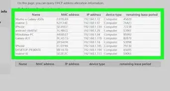
3Press the Ctrl or ⌘ Cmd key as you click. All the cells you click will be added to your selection when you have that key pressed.
- You can release the key when you are done making your selections.
-
4Click View. You'll see this either in the editing ribbon above the document space or at the top of your screen.
-
5Click Freeze Panes. A menu will dropdown.
-
6Click Freeze Panes. This will freeze the panes in the columns next to what you have selected.[4]
- You'll notice when you freeze panes if you scroll away and a column or row stays on the screen.


Unfreezing Panes
-
1Open your project in Excel. You can either open the program within Excel by clicking File > Open, or you can right-click the file in your file explorer.
-
2Go to View. You'll see a drop-down menu.
-
3Click Freeze Panes. It's next to Arrange All and Split/Hide towards the right side of the toolbar.
-
4Click Unfreeze Panes. This will unfreeze all the cells that you have frozen on the screen.


References
- ↑ https://support.office.com/en-us/article/freeze-panes-to-lock-the-first-row-or-column-in-excel-for-mac-b8eb717e-9d3e-4354-8c02-d779a4b404b2
- ↑ https://support.office.com/en-us/article/freeze-panes-to-lock-rows-and-columns-dab2ffc9-020d-4026-8121-67dd25f2508f
- ↑ https://support.office.com/en-us/article/freeze-panes-to-lock-the-first-row-or-column-in-excel-for-mac-b8eb717e-9d3e-4354-8c02-d779a4b404b2
- ↑ https://support.office.com/en-us/article/freeze-panes-to-lock-rows-and-columns-dab2ffc9-020d-4026-8121-67dd25f2508f
About This Article

1. Open your project in Excel.
2. Select cell to the right of the column you want to freeze.
3. Click View.
4. Click Freeze Panes.
5. Click Freeze Panes.