This article was co-authored by wikiHow Staff. Our trained team of editors and researchers validate articles for accuracy and comprehensiveness. wikiHow's Content Management Team carefully monitors the work from our editorial staff to ensure that each article is backed by trusted research and meets our high quality standards.
The wikiHow Tech Team also followed the article's instructions and verified that they work.
This article has been viewed 49,727 times.
Learn more...
This wikiHow teaches you how to change the name or value of a chart's legend entries in a Microsoft Excel spreadsheet, using a computer.
Steps
-
1Open the Excel spreadsheet file you want to edit. Find the spreadsheet you want to edit on your computer, and double-click on its icon to open the worksheet.
-
2Click on the chart you want to edit. Find the chart you want to modify in your spreadsheet, and click on it to select the chart.
- This will display your chart tool tabs at the top of your spreadsheet, such as Design, Layout, and Format
Advertisement -
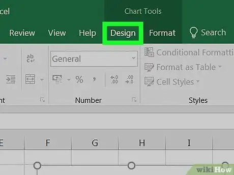
3Click the Design tab. You can find it at the top of Excel's toolbar ribbon. It will display your chart design tools on the toolbar.
- Depending on your version of Excel, this tab may be named Chart Design.
-
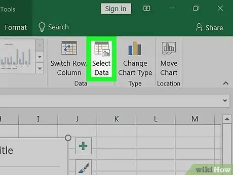
4Click Select Data in the Design toolbar. This will open a new dialogue box where you can edit your legend and data values.
-
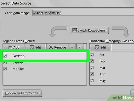
5Select a legend entry in the "Legend entries (Series)" box. This box lists all the legend entries in your chart. Find the entry you want to edit here, and click on it to select it.
-
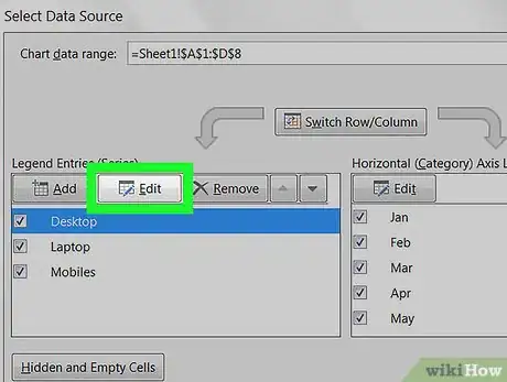
6Click the Edit button. This will allow you to edit the selected entry's name and data values.
- On some versions of Excel, you won't see an Edit button. In this case, you can skip this step, and look for the Name or Series Name field in the same dialogue box.
-
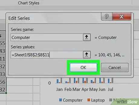
7Type in a new entry name into the Series Name box. Double-click the text field, delete the current name, and enter the name you want to assign to this entry in your chart's legend.
- This box may also be labeled as Name instead of Series Name.
- Alternatively, you can click the Collapse Dialogue icon, and select a cell from the spreadsheet. This will copy and assign the selected cell's contents as the entry name.
-
8Enter a new chart value into the Y values box. You can delete the selected entry's current value here, and type in a new value to change your chart.
- If you have multiple Y output categories in your chart, such as multiple bars, make sure to use a comma to separate each value here.
- Alternatively, you can click the Collapse Dialogue icon, and select a cell or multiple cells from the spreadsheet to import the cell values into your chart.
-
9Click the OK button. This will save your name and value edits, and apply the changes to your visual chart.
About This Article
1. Open a spreadsheet, and click the chart you want to edit.
2. Click the Design or Chart Design tab.
3. Click Select Data on the toolbar.
4. Select a legend entry, and click Edit.
5. Enter a new name into the Series Name or Name box.
6. Enter a new value into the Y values box.
7. Click OK.


