This article was co-authored by wikiHow staff writer, Nicole Levine, MFA. Nicole Levine is a Technology Writer and Editor for wikiHow. She has more than 20 years of experience creating technical documentation and leading support teams at major web hosting and software companies. Nicole also holds an MFA in Creative Writing from Portland State University and teaches composition, fiction-writing, and zine-making at various institutions.
The wikiHow Tech Team also followed the article's instructions and verified that they work.
This article has been viewed 488,035 times.
Learn more...
Do you want to add more information to your pivot table without altering your source data? You easily can add custom calculated fields to create formulas within the pivot table instead of adding more columns to your worksheet. Custom fields can do nearly any calculations you need, like displaying averages, percentages, variances, and maximum values for fields. We'll walk you through adding a custom calculated field to a pivot table in your Microsoft Excel spreadsheet, and show you how to edit the field any time you need to change the formula.
Steps
Adding Custom Fields
-
1Open your workbook. Double-click the file that has the source data and pivot table you'll be working with.
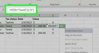
- Keep in mind that calculated fields can't use references or named ranges in formulas—this means you can't use functions like INDEX, OFFSET, or VLOOKUP in your custom field. However, functions like IF, SUM, COUNT, and any others that don't require references or named ranges are fine.
-
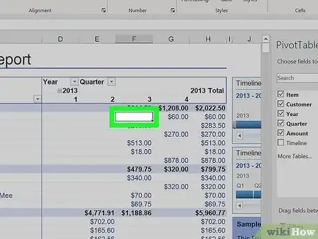
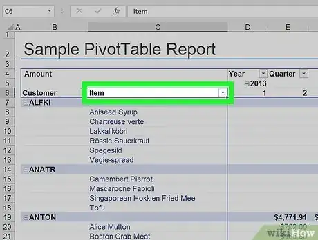
2Click the pivot table you want to edit. When you click the pivot table, the "PivotTable Fields" panel will expand on the right. You'll also see the PivotTable Analyze menu at the top of Excel.Advertisement
-
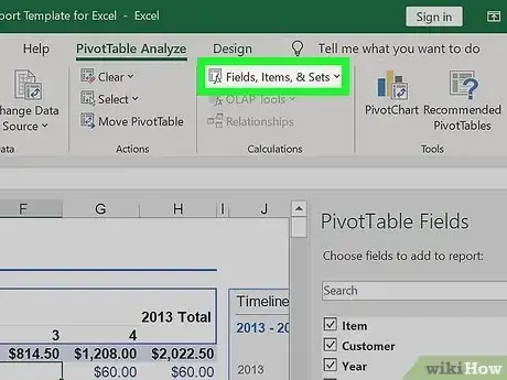
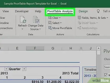
3Click the PivotTable Analyze tab. You'll see this tab at the top of Excel.
- The PivotTable Analyze menu is only visible when you click to activate the pivot table. If the menu ever disappears, just click the pivot table again to bring it back up.
- This tab is called Analyze in some versions of Excel.
-
4Click the Fields, Items, & Sets menu. You'll see this in the "Calculations" area of the toolbar at the top of Excel.
-
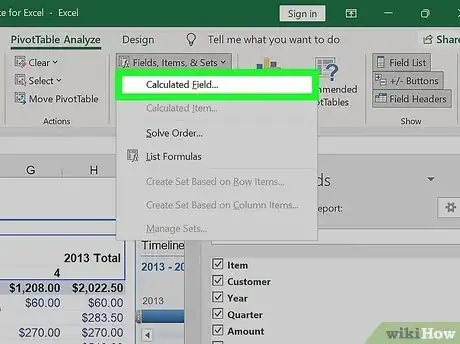
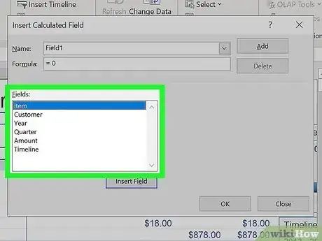
5Click Calculated Field…. Once you click this menu option, the "Insert Calculated Field" dialog box will appear.[1]
-
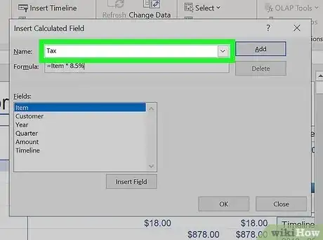
6Enter a name for the field. Type a descriptive column label for your custom field into the "Name" box.
-
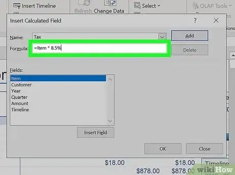
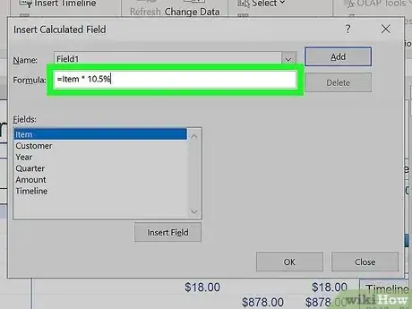
7Create a formula for your custom field. In the "Formula" box, type the formula you want to use to calculate your custom field.
- For example, to find the tax rate for the "Items" field at 8.5%, you could name your custom field "Tax" and use this formula:=Items * 8.5%.
- Another example: If you want to divide values in the "Sales" column by values in the "Quantity" column, you could use: =Sales/Quantity.
- To insert data from another pivot table field in your formula, select the field and click Insert Field.
-
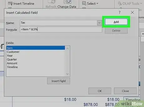
8Click Add. This adds your custom field to the Fields list.
-
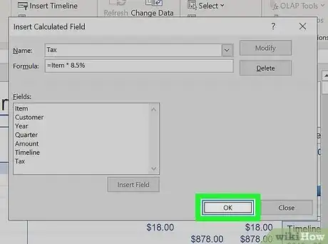
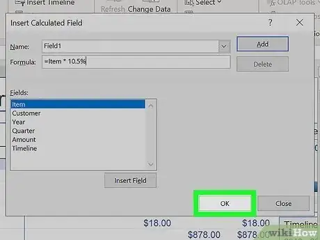
9Click OK. This closes the "Insert Calculated Field" box and returns you to the pivot table.
-
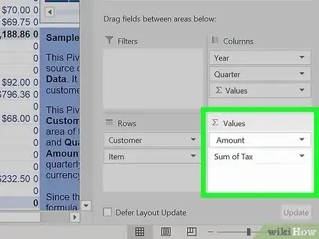
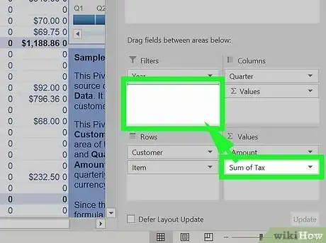
10Find your new field in the "Values" area. Now that you've added a new field, you'll see it in the "PivotTable Fields" panel on the right side of your sheet in the "Values" column.
-
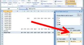
11Drag your new field to the desired area. You can now drag your custom calculated field from the Values area to Filters, Rows, or Columns to apply the formula to your data.
Editing Custom Fields
-
1Select the pivot table containing the field you want to edit. Editing the formula in this one calculated field is much easier than creating—and later editing—a formula in the source data. This can be useful when the amount by which you are calculating your field changes often. Clicking the pivot table will activate the PivotTable Analyze or Analyze menu at the top of Excel.
-
2Click the PivotTable Analyze or Analyze tab. You'll see these at the top of Excel.
-
3Click the Fields, Items, & Sets menu. You'll see this in the "Calculations" area of the toolbar at the top of Excel.
-
4Click Calculated Field…. Once you click this menu option, the "Insert Calculated Field" dialog box will appear.
-
5Select the field you want to edit. All fields, including your custom fields, appear in the "Fields" area. When you click your custom field, you'll see its formula in the "Formula" box, and its name in the "Name" box.
-
6Modify the field's name or formula. You can now make any adjustments you need to your custom field.
- If you want to delete the field, just click Delete instead.
-
7Click OK. Your field is now updated. If your pivot table doesn't refresh automatically, right-click the table and select Refresh to see your new calculations.
Expert Q&A
-
QuestionEvery time that I create a new pivot table and I select a field (revenue) and I move it to values space, it defaults to count of revenue even though I've used sum of revenue in previous pivot tables.
 Nicole Levine, MFANicole Levine is a Technology Writer and Editor for wikiHow. She has more than 20 years of experience creating technical documentation and leading support teams at major web hosting and software companies. Nicole also holds an MFA in Creative Writing from Portland State University and teaches composition, fiction-writing, and zine-making at various institutions.
wikiHow Technology Writer It would default to count instead of sum if there are any blank cells or errors in your data--if you have any of either, replace them with 0 (zeros) and that should sort if out. If that doesn't work, you might have non-numerical characters in your data (or numbers that are formatted as text instead of numbers). Make sure your data is purely numerical and you should get a sum instead of the count.
 -
QuestionHow can I add a new field to the Filters or Rows section of the Pivot Table?
 Nicole Levine, MFANicole Levine is a Technology Writer and Editor for wikiHow. She has more than 20 years of experience creating technical documentation and leading support teams at major web hosting and software companies. Nicole also holds an MFA in Creative Writing from Portland State University and teaches composition, fiction-writing, and zine-making at various institutions.
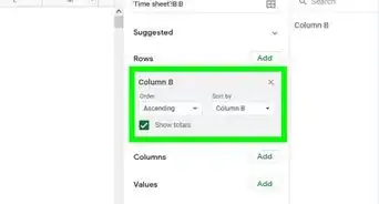
wikiHow Technology Writer Once you create the new field, it will appear in the "Values" section of the PivotTable Fields panel on the right side of your sheet. To use the value as a filter, drag it over to the Filters section.
 -
QuestionI would like to display the number of occurrences (count) of incidences where where column A is less than 100 when Column C is equal to a given value.
 Nicole Levine, MFANicole Levine is a Technology Writer and Editor for wikiHow. She has more than 20 years of experience creating technical documentation and leading support teams at major web hosting and software companies. Nicole also holds an MFA in Creative Writing from Portland State University and teaches composition, fiction-writing, and zine-making at various institutions.
wikiHow Technology Writer The COUNTIFS formula would get you that result, but you can't use that function in a calculated field. You might want to add a new column to your source data that contains an IFS statement, which you can count in your pivot table without adding any calculated fields.

