The One-Way F-Test

The $F$ test as a one-way analysis of variance is used to assess whether the expected values of a quantitative variable within several pre-defined groups differ from each other. For example, suppose that a medical trial compares four treatments. The ANOVA $F$-test can be used to assess whether any of the treatments is on average superior, or inferior, to the others versus the null hypothesis that all four treatments yield the same mean response. This is an example of an "omnibus" test, meaning that a single test is performed to detect any of several possible differences.

Alternatively, we could carry out pairwise tests among the treatments (for instance, in the medical trial example with four treatments we could carry out six tests among pairs of treatments). The advantage of the ANOVA $F$-test is that we do not need to pre-specify which treatments are to be compared, and we do not need to adjust for making multiple comparisons. The disadvantage of the ANOVA $F$-test is that if we reject the null hypothesis, we do not know which treatments can be said to be significantly different from the others. If the $F$-test is performed at level $\alpha$ we cannot state that the treatment pair with the greatest mean difference is significantly different at level $\alpha$.

The formula for the one-way ANOVA $F$-test statistic is:

$F=\dfrac { \text{explained variance} }{ \text{unexplained variance} }$

or

$F=\dfrac { \text{between-group variability} }{ \text{within-group variability} }$

The "explained variance," or "between-group variability" is:

$\displaystyle \sum _{ i }^{ } \frac{{ n }_{ i }{ \left( { \bar { Y } }_{ i }-\bar { Y } \right) }^{ 2 }}{\left( K-1 \right)}$

where ${ \bar { Y } }_{ i }$ denotes the sample mean in the $i$^th group, $n_i$ is the number of observations in the $i$^th group, $\bar { Y }$ denotes the overall mean of the data, and $K$ denotes the number of groups.

The "unexplained variance", or "within-group variability" is:

$\displaystyle \sum _{ ij }^{ }\frac{{ \left( { \bar { Y } }_{ ij }-{ \bar { Y } }_{ i } \right) }^{ 2 }} {\left( N-K \right)}$

where $\bar{Y_{ij}}$ is the $j$^th observation in the $i$^th out of $K$ groups and $N$ is the overall sample size. This $F$-statistic follows the $F$-distribution with $K-1$, $N-K$ degrees of freedom under the null hypothesis. The statistic will be large if the between-group variability is large relative to the within-group variability, which is unlikely to happen if the population means of the groups all have the same value.

Note that when there are only two groups for the one-way ANOVA $F$-test, $F=t^2$ where $t$ is the Student's $t$-statistic.

Example

Four sororities took a random sample of sisters regarding their grade means for the past term. The data were distributed as follows:

• Sorority 1: 2.17, 1.85, 2.83, 1.69, 3.33
• Sorority 2: 2.63,1.77, 3.25, 1.86, 2.21
• Sorority 3: 2.63, 3.78, 4.00, 2.55, 2.45
• Sorority 4: 3.79, 3.45, 3.08, 2.26, 3.18

Using a significance level of 1%, is there a difference in mean grades among the sororities?

Solution

Let $\mu_1$, $\mu_2$, $\mu_3$, $\mu_4$ be the population means of the sororities. Remember that the null hypothesis claims that the sorority groups are from the same normal distribution. The alternate hypothesis says that at least two of the sorority groups come from populations with different normal distributions. Notice that the four sample sizes are each size 5. Also, note that this is an example of a balanced design, since each factor (i.e., sorority) has the same number of observations.

$H_0: \mu_1 = \mu_2 = \mu_3 = \mu_4$

$H_a:$ Not all of the means $\mu_1$, $\mu_2$, $\mu_3$, $\mu_4$ are equal

Distribution for the test: $F_{3, 16}$

where $k=4$ groups and $n=20$ samples in total

$df_{\text{numerator}} = k-1 = 4-1 = 3$

$df_{\text{denominator}} = n-k = 20-4 = 16$

Calculate the test statistic: $F=2.23$

Graph:

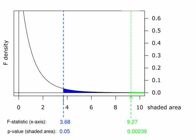
Graph of $p$-Value

This chart shows example p-values for two F-statistics: p = 0.05 for F = 3.68, and p = 0.00239 for F = 9.27. These numbers are evidence of the skewness of the F-curve to the right; a much higher F-value corresponds to an only slightly smaller p-value.

Probability statement: $p\text{-value} = P(F>2.23) = 0.1241$

Compare $\alpha$ and the $p$-value: $\alpha = 0.01$, $p\text{-value} = 0.1241$

Make a decision: Since $\alpha < p\text{-value}$, you cannot reject $H_0$.

Conclusion: There is not sufficient evidence to conclude that there is a difference among the mean grades for the sororities.