Statistics
Textbooks
Boundless Statistics
Estimation and Hypothesis Testing
Hypothesis Testing: Two Samples
Statistics Textbooks Boundless Statistics Estimation and Hypothesis Testing Hypothesis Testing: Two Samples
Statistics Textbooks Boundless Statistics Estimation and Hypothesis Testing
Statistics Textbooks Boundless Statistics
Statistics Textbooks
Statistics
Concept Version 7
Created by Boundless

Comparing Two Population Variances

In order to compare two variances, we must use the $F$ distribution.

Learning Objective

  • Outline the $F$-test and how it is used to test two population variances.


Key Points

    • In order to perform a $F$ test of two variances, it is important that the following are true: (1) the populations from which the two samples are drawn are normally distributed, and (2) the two populations are independent of each other.
    • When we are interested in comparing the two sample variances, we use the $F$ ratio: $F=\dfrac { \left[ \dfrac { { s }_{ 1 }^{ 2 } }{ { \sigma }_{ 1 }^{ 2 } } \right] }{ \left[ \dfrac { { s }_{ 2 }^{ 2 } }{ { \sigma }_{ 2 }^{ 2 } } \right] }$.
    • If the null hypothesis is $\sigma_1^2 = \sigma_2^2$, then the $F$ ratio becomes: $F=\dfrac { \left[ \dfrac { { s }_{ 1 }^{ 2 } }{ { \sigma }_{ 1 }^{ 2 } } \right] }{ \left[ \dfrac { { s }_{ 2 }^{ 2 } }{ { \sigma }_{ 2 }^{ 2 } } \right] } =\dfrac { { s }_{ 1 }^{ 2 } }{ { s }_{ 2 }^{ 2 } }$.
    • If the two populations have equal variances the $F$ ratio is close to 1.
    • If the two population variances are far apart the $F$ ratio becomes a large number.
    • Therefore, if $F$ is close to 1, the evidence favors the null hypothesis (the two population variances are equal); but if $F$ is much larger than 1, then the evidence is against the null hypothesis.

Terms

  • F distribution

    A probability distribution of the ratio of two variables, each with a chi-square distribution; used in analysis of variance, especially in the significance testing of a correlation coefficient ($R$ squared).

  • null hypothesis

    A hypothesis set up to be refuted in order to support an alternative hypothesis; presumed true until statistical evidence in the form of a hypothesis test indicates otherwise.


Full Text

It is often desirable to compare two variances, rather than two means or two proportions. For instance, college administrators would like two college professors grading exams to have the same variation in their grading. In order for a lid to fit a container, the variation in the lid and the container should be the same. A supermarket might be interested in the variability of check-out times for two checkers. In order to compare two variances, we must use the $F$ distribution.

In order to perform a $F$ test of two variances, it is important that the following are true:

  1. The populations from which the two samples are drawn are normally distributed.
  2. The two populations are independent of each other.

Suppose we sample randomly from two independent normal populations. Let $\sigma_1^2$ and $\sigma_2^2$ be the population variances and $s_1^2$ and $s_2^2$ be the sample variances. Let the sample sizes be $n_1$ and $n_2$. Since we are interested in comparing the two sample variances, we use the $F$ ratio:

$F=\dfrac { \left[ \dfrac { { s }_{ 1 }^{ 2 } }{ { \sigma }_{ 1 }^{ 2 } } \right] }{ \left[ \dfrac { { s }_{ 2 }^{ 2 } }{ { \sigma }_{ 2 }^{ 2 } } \right] }$

$F$ has the distribution $F \sim F(n_1 - 1, n_2 - 1)$ where $n_1 - 1$ are the degrees of freedom for the numerator and $n_2 - 1$ are the degrees of freedom for the denominator.

If the null hypothesis is $\sigma_1^2 = \sigma_2^2$, then the $F$ ratio becomes:

 $F=\dfrac { \left[ \dfrac { { s }_{ 1 }^{ 2 } }{ { \sigma }_{ 1 }^{ 2 } } \right] }{ \left[ \dfrac { { s }_{ 2 }^{ 2 } }{ { \sigma }_{ 2 }^{ 2 } } \right] } =\dfrac { { s }_{ 1 }^{ 2 } }{ { s }_{ 2 }^{ 2 } }$

Note that the $F$ ratio could also be $\frac { { s }_{ 2 }^{ 2 } }{ { s }_{ 1 }^{ 2 } }$. It depends on $H_a$ and on which sample variance is larger.

If the two populations have equal variances, then $s_1^2$ and $s_2^2$ are close in value and $F=\frac { { s }_{ 1 }^{ 2 } }{ { s }_{ 2 }^{ 2 } }$ is close to 1. But if the two population variances are very different, $s_1^2$ and $s_2^2$ tend to be very different, too. Choosing $s_1^2$ as the larger sample variance causes the ratio $\frac { { s }_{ 1 }^{ 2 } }{ { s }_{ 2 }^{ 2 } }$ to be greater than 1. If $s_1^2$ and $s_2^2$ are far apart, then $F=\frac { { s }_{ 1 }^{ 2 } }{ { s }_{ 2 }^{ 2 } }$ is a large number.

Therefore, if $F$ is close to 1, the evidence favors the null hypothesis (the two population variances are equal). But if $F$ is much larger than 1, then the evidence is against the null hypothesis.

A test of two variances may be left, right, or two-tailed.

Example

Two college instructors are interested in whether or not there is any variation in the way they grade math exams. They each grade the same set of 30 exams. The first instructor's grades have a variance of 52.3. The second instructor's grades have a variance of 89.9.

Test the claim that the first instructor's variance is smaller. (In most colleges, it is desirable for the variances of exam grades to be nearly the same among instructors.) The level of significance is 10%.

Solution

Let 1 and 2 be the subscripts that indicate the first and second instructor, respectively: $n_1 = n_2 = 30$.

$H_0: \sigma_1^2 = \sigma_2^2$ and $H_a: \sigma_1^2 < \sigma_2^2$

Calculate the test statistic: By the null hypothesis ($\sigma_1^2 = \sigma_2^2$), the F statistic is:

$\displaystyle F=\frac { \left[ \frac { { s }_{ 1 }^{ 2 } }{ { \sigma }_{ 1 }^{ 2 } } \right] }{ \left[ \frac { { s }_{ 2 }^{ 2 } }{ { \sigma }_{ 2 }^{ 2 } } \right] } =\frac { { s }_{ 1 }^{ 2 } }{ { s }_{ 2 }^{ 2 } } =\frac { 52.3 }{ 89.9 } =0.6$

Distribution for the test: $F_{29, 29}$ where $n_1-1 = 29$ and $n_2 -1 = 29$.

Graph: This test is left-tailed:
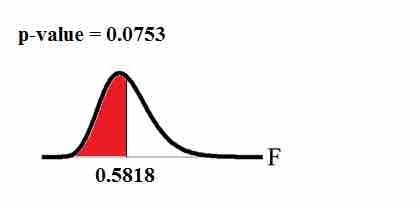
$p$-Value Graph

This image shows the graph of the $p$-value we calculate in our example.

Probability statement: $p\text{-value} = P(F<0.5818) = 0.0753$.

Compare $\alpha$ and the $p$-value: $\alpha = 0.10 > p\text{-value}$.

Make a decision: Since $\alpha > p\text{-value}$, reject $H_0$.

Conclusion: With a 10% level of significance, from the data, there is sufficient evidence to conclude that the variance in grades for the first instructor is smaller.

[ edit ]
Edit this content
Prev Concept
Comparing Matched or Paired Samples
Determining Sample Size
Next Concept
Subjects
  • Accounting
  • Algebra
  • Art History
  • Biology
  • Business
  • Calculus
  • Chemistry
  • Communications
  • Economics
  • Finance
  • Management
  • Marketing
  • Microbiology
  • Physics
  • Physiology
  • Political Science
  • Psychology
  • Sociology
  • Statistics
  • U.S. History
  • World History
  • Writing

Except where noted, content and user contributions on this site are licensed under CC BY-SA 4.0 with attribution required.