Comparing Matched or Paired Samples

When performing a hypothesis test comparing matched or paired samples, the following points hold true:

1. Simple random sampling is used.
2. Sample sizes are often small.
3. Two measurements (samples) are drawn from the same pair of individuals or objects.
4. Differences are calculated from the matched or paired samples.
5. The differences form the sample that is used for the hypothesis test.
6. The matched pairs have differences arising either from a population that is normal, or because the number of differences is sufficiently large so the distribution of the sample mean of differences is approximately normal.

In a hypothesis test for matched or paired samples, subjects are matched in pairs and differences are calculated. The differences are the data. The population mean for the differences, $\mu_d$, is then tested using a Student-$t$ test for a single population mean with $n-1$ degrees of freedom, where $n$ is the number of differences.

The test statistic ($t$-score) is:

$t=\dfrac { \bar { { x }_{ d } } -{ \mu }_{ d } }{ \left( \dfrac { { s }_{ d } }{ \sqrt { n } } \right) }$

Example

A study was conducted to investigate the effectiveness of hypnotism in reducing pain. Results for randomly selected subjects are shown in the table below. The "before" value is matched to an "after" value, and the differences are calculated. The differences have a normal distribution .

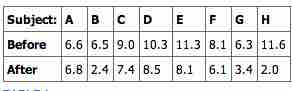
Paired Samples Table 1

This table shows the before and after values of the data in our sample.

Are the sensory measurements, on average, lower after hypnotism? Test at a 5% significance level.

Solution

shows that the corresponding "before" and "after" values form matched pairs. (Calculate "after" minus "before").

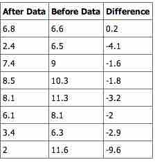
Paired Samples Table 2

This table shows the before and after values and their calculated differences.

The data for the test are the differences:

{0.2, -4.1, -1.6, -1.8, -3.2, -2, -2.9, -9.6}

The sample mean and sample standard deviation of the differences are: \bar { { x }_{ d } } =-3.13 and 

Verify these values. Let μ_d be the population mean for the differences. We use the subscript d to denote "differences".

Random Variable: $\bar { { x }_{ d } }$ (the mean difference of the sensory measurements):

${ H }_{ 0 }:{ \mu }_{ d }\ge 0$

There is no improvement. ($\mu_d$ is the population mean of the differences.)

${ H }_{ a }:{ \mu }_{ d }<0$

There is improvement. The score should be lower after hypnotism, so the difference ought to be negative to indicate improvement.

Distribution for the test: The distribution is a student-$t$ with $df = n-1 = 8-1 = 7$. Use $t_7$. (Notice that the test is for a single population mean. )

Calculate the $p$-value using the Student-$t$ distribution: $p\text{-value} = 0.0095$

Graph:

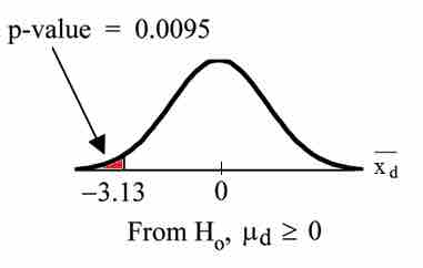
$p$-Value Graph

This image shows the graph of the $p$-value obtained in our example.

$\bar { { X }_{ d } }$ is the random variable for the differences. The sample mean and sample standard deviation of the differences are:

$\bar { { x }_{ d } } =-3.13$

$\bar { { s }_{ d } } =2.91$

Compare $\alpha$ and the $p$-value: $\alpha = 0.05$ and $p\text{-value} = 0.0095$. $\alpha > p\text{-value}$.

Make a decision: Since $\alpha > p\text{-value}$, reject $H_0$. This means that $\mu_d < 0 $, and there is improvement.

Conclusion: At a 5% level of significance, from the sample data, there is sufficient evidence to conclude that the sensory measurements, on average, are lower after hypnotism. Hypnotism appears to be effective in reducing pain.