Chemistry
Textbooks
Boundless Chemistry
Chemical Kinetics
The Rate Law: Concentration and Time
Chemistry Textbooks Boundless Chemistry Chemical Kinetics The Rate Law: Concentration and Time
Chemistry Textbooks Boundless Chemistry Chemical Kinetics
Chemistry Textbooks Boundless Chemistry
Chemistry Textbooks
Chemistry
Concept Version 10
Created by Boundless

The Integrated Rate Law

The integrated rate laws derive from calculus, and they relate the concentrations of reactants with time.

Learning Objective

  • Graph integrated rate laws for zero-, first-, and second-order reactions in order to obtain information about the rate constant and concentrations of reactants


Key Points

    • Each reaction order rate equation can be integrated to relate time and concentration.
    • A plot of 1/[A] versus t yields a straight line with a slope of k for a second-order reaction.
    • A plot of ln[A] versus t yields a straight line with a slope of -k for a first-order reaction.
    • A plot of [A] versus t gives a straight line with a slope of -k for a zero-order reaction.

Term

  • integrated rate equation

    Links concentrations of reactants or products with time; integrated from the rate law.


Full Text

The rate law is a differential equation, meaning that it describes the change in concentration of reactant(s) per change in time. Using calculus, the rate law can be integrated to obtain an integrated rate equation that links concentrations of reactants or products with time directly.

Integrated Raw Law for a First-Order Reaction

Recall that the rate law for a first-order reaction is given by:

$rate = -\frac{d[A]}{dt}=k[A]$

We can rearrange this equation to combine our variables, and integrate both sides to get our integrated rate law:

$\int^{[A]_t}_{[A]_0} \frac{d[A]}{[A]}=-\int^t_0k\;dt$

$ln\left(\frac{[A]_t}{[A]_0}\right)=-kt$

$\frac{[A]_t}{[A]_0}=e^{-kt}$

Finally, putting this equation in terms of $[A]_t$, we have:

$[A]_t=[A]_0e^{-kt}$

This is the final form of the integrated rate law for a first-order reaction. Here, [A]t represents the concentration of the chemical of interest at a particular time t, and [A]0 represents the initial concentration of A. Note that this equation can also be written in the following form:

$ln[A]=-kt+ln[A]_0$

This form is useful, because it is of the form $y=mx+b$. When the integrated rate law is written in this way, a plot of $ln[A]$ versus t will yield a straight line with the slope -k. However, the integrated first-order rate law is usually written in the form of the exponential decay equation.

Integrated Rate Law for a Second-Order Reaction

Recall that the rate law for a second-order reaction is given by:

$rate=-\frac{d[A]}{dt}=k[A]^2$

Rearranging our variables and integrating, we get the following:

$\int^{[A]_t}_{[A]_0}\frac{d[A]}{[A]^2}=-\int^t_0 k\;dt$

$\frac{1}{[A]_t}-\frac{1}{[A]_0}=kt$

The final version of this integrated rate law is given by:

$\frac{1}{[A]_t}=\frac{1}{[A]_0}+kt$

Note that this equation is also of the form $y=mx+b$. Here, a plot of $\frac{1}{[A]}$ versus t will yield a straight line with a positive slope k.

Integrated Rate Law for Second-Order Reaction with Two Reactants

For a reaction that is second-order overall, and first-order in two reactants, A and B, our rate law is given by:

$rate=-\frac{d[A]}{dt}=-\frac{d[B]}{dt}=k[A][B]$

There are two possible scenarios here. The first is that the initial concentrations of A and B are equal, which simplifies things greatly. In this case, we can say that [A]=[B], and the rate law simplifies to:

$rate=k[A]^2$

This is the standard form for second-order rate law, and the integrated rate law will be the same as above. However, in the case where $[A]_0\neq [B]_0$ , the integrated rate law will take the form:

$ln\frac{[B][A]_0}{[A][B]_0}=k([B]_0-[A]_0)t$

In this more complicated instance, a plot of $ln\frac{[B][A]_0}{[A][B]_0}$ versus t will yield a straight line with a slope of $k([B]_0-[A]_0)$.

Integrated Rate Law for a Zero-Order Reaction

The rate law for a zero-order reaction is given by:

$rate=-\frac{d[A]}{dt}=k$

Rearranging and integrating, we have:

$\int^{[A]_t}_{[A]_0}d[A]=-\int^t_0 k\;dt$

$[A]_t-[A]_0=-kt$

$[A]_t=-kt+[A]_0$

Note here that a plot of [A] versus t will yield a straight line with the slope -k. The y-intercept of this plot will be the initial concentration of A, [A]0.

Summary

The important thing is not necessarily to be able to derive each integrated rate law from calculus, but to know the forms, and which plots will yield straight lines for each reaction order. A summary of the various integrated rate laws, including the different plots that will yield straight lines, can be used as a resource.

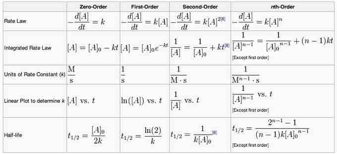
Summary of integrated rate laws for zero-, first-, second-, and nth-order reactions

A summary of reactions with the differential and integrated equations.

[ edit ]
Edit this content
Prev Concept
Zero-Order Reactions
Half-Life
Next Concept
Subjects
  • Accounting
  • Algebra
  • Art History
  • Biology
  • Business
  • Calculus
  • Chemistry
  • Communications
  • Economics
  • Finance
  • Management
  • Marketing
  • Microbiology
  • Physics
  • Physiology
  • Political Science
  • Psychology
  • Sociology
  • Statistics
  • U.S. History
  • World History
  • Writing

Except where noted, content and user contributions on this site are licensed under CC BY-SA 4.0 with attribution required.