McNemar's test is a normal approximation used on nominal data. It is applied to
A contingency table used in McNemar's test tabulates the outcomes of two tests on a sample of
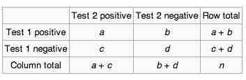
$2 \times 2$ Contingency Table
A contingency table used in McNemar's test tabulates the outcomes of two tests on a sample of
The null hypothesis of marginal homogeneity states that the two marginal probabilities for each outcome are the same, i.e.
Here
Under the null hypothesis, with a sufficiently large number of discordants,
If the