Comparing Two Independent Population Means

Independent samples are simple random samples from two distinct populations. To compare these random samples, both populations are normally distributed with the population means and standard deviations unknown unless the sample sizes are greater than 30. In that case, the populations need not be normally distributed.

The comparison of two population means is very common. The difference between the two samples depends on both the means and the standard deviations. Very different means can occur by chance if there is great variation among the individual samples. In order to account for the variation, we take the difference of the sample means,

$\bar { { X }_{ 1 } } -\bar { { X }_{ 2 } }$

and divide by the standard error (shown below) in order to standardize the difference. The result is a $t$-score test statistic (also shown below).

Because we do not know the population standard deviations, we estimate them using the two sample standard deviations from our independent samples. For the hypothesis test, we calculate the estimated standard deviation, or standard error, of the difference in sample means,

$\bar { { X }_{ 1 } } -\bar { { X }_{ 2 } }$.

The standard error is:

$\displaystyle \sqrt { \frac { { S }_{ 1 }^{ 2 } }{ { n }_{ 1 } } +\frac { { S }_{ 2 }^{ 2 } }{ { n }_{ 2 } } }$.

The test statistic ($t$-score) is calculated as follows:

$\dfrac { (\bar { { X }_{ 1 } } -\bar { { X }_{ 2 } } )-({ \mu }_{ 1 }-{ \mu }_{ 2 }) }{ \sqrt { \dfrac { { S }_{ 1 }^{ 2 } }{ { n }_{ 1 } } +\dfrac { { S }_{ 2 }^{ 2 } }{ { n }_{ 2 } } } }$.

The degrees of freedom ($df$) is a somewhat complicated calculation. The $df$s are not always a whole number. The test statistic calculated above is approximated by the student's-$t$ distribution with $df$s as follows:

$\displaystyle df=\frac { { \left( \frac { { S }_{ 1 }^{ 2 } }{ { n }_{ 1 } } +\frac { { S }_{ 2 }^{ 2 } }{ { n }_{ 2 } } \right) }^{ 2 } }{ \left[ \left( \frac { 1 }{ { n }_{ 1 } } -1 \right) \cdot { \left( \frac { { S }_{ 1 }^{ 2 } }{ { n }_{ 1 } } \right) }^{ 2 }+\left( \frac { 1 }{ { n }_{ 2 } } -1 \right) \cdot { \left( \frac { { S }_{ 2 }^{ 2 } }{ { n }_{ 2 } } \right) }^{ 2 } \right] }$

Note that it is not necessary to compute this by hand. A calculator or computer easily computes it.

Example

The average amount of time boys and girls ages 7 through 11 spend playing sports each day is believed to be the same. An experiment is done, data is collected, resulting in the table below. Both populations have a normal distribution. 

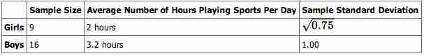
Independent Sample Table 1

This table lays out the parameters for our example.

Is there a difference in the mean amount of time boys and girls ages 7 through 11 play sports each day? Test at the 5% level of significance.

Solution

The population standard deviations are not known. Let $g$ be the subscript for girls and $b$ be the subscript for boys. Then, $\mu_g$ is the population mean for girls and $\mu_b$ is the population mean for boys. This is a test of two independent groups, two population means.

The random variable: $\bar { { X }_{ g } } -\bar { { X }_{ b } }$ is the difference in the sample mean amount of time girls and boys play sports each day.

$H_0: \mu_g = \mu_{bg-b} = 0$

$H_a: \mu_g \neq \mu_{bg-b} \neq 0$

The words "the same" tell you $H_0$ has an "=". Since there are no other words to indicate $H_a$, then assume "is different." This is a two-tailed test.

Distribution for the test: Use $t_{df}$ where $df$ is calculated using the $df$ formula for independent groups, two population means. Using a calculator, $df$ is approximately 18.8462.

Calculate the $p$-value using a student's-$t$ distribution: $p\text{-value} = 0.0054$

Graph:

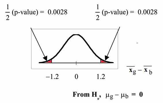
Graph for Example

This image shows the graph for the $p$-values in our example.

${ s }_{ g }=\sqrt { 0.75 }$

${ s }_{ b }=1$

so, $\bar { { X }_{ g } } -\bar { { X }_{ b } }=2-3.1=-1.2$

Half the $p$-value is below $-1.2$ and half is above 1.2.

Make a decision: Since $\alpha > p\text{-value}$, reject $H_0$. This means you reject $\mu_g = \mu_b$. The means are different.

Conclusion: At the 5% level of significance, the sample data show there is sufficient evidence to conclude that the mean number of hours that girls and boys aged 7 through 11 play sports per day is different (the mean number of hours boys aged 7 through 11 play sports per day is greater than the mean number of hours played by girls OR the mean number of hours girls aged 7 through 11 play sports per day is greater than the mean number of hours played by boys).