A test of a single variance assumes that the underlying distribution is normal. The null and alternate hypotheses are stated in terms of the population variance (or population standard deviation). The test statistic is:
where:
We may think of
A test of a single variance may be right-tailed, left-tailed, or two-tailed.
The following example shows how to set up the null hypothesis and alternate hypothesis. The null and alternate hypotheses contain statements about the population variance.
Example 1
Math instructors are not only interested in how their students do on exams, on average, but how the exam scores vary. To many instructors, the variance (or standard deviation) may be more important than the average.
Suppose a math instructor believes that the standard deviation for his final exam is 5 points. One of his best students thinks otherwise. The student claims that the standard deviation is more than 5 points. If the student were to conduct a hypothesis test, what would the null and alternate hypotheses be?
Solution
Even though we are given the population standard deviation, we can set the test up using the population variance as follows.
Example 2
With individual lines at its various windows, a post office finds that the standard deviation for normally distributed waiting times for customers on Friday afternoon is 7.2 minutes. The post office experiments with a single main waiting line and finds that for a random sample of 25 customers, the waiting times for customers have a standard deviation of 3.5 minutes.
With a significance level of 5%, test the claim that a single line causes lower variation among waiting times (shorter waiting times) for customers.
Solution
Since the claim is that a single line causes lower variation, this is a test of a single variance. The parameter is the population variance,
Random Variable: The sample standard deviation,
-
${ H }_{ 0 }={ \sigma }^{ 2 }={ 7.2 }^{ 2 }$ -
${ H }_{ a }={ \sigma }^{ 2 }<{ 7.2 }^{ 2 }$
The word "lower" tells you this is a left-tailed test.
Distribution for the test:
-
$n$ is the number of customers sampled -
$df = n-1 = 25-1 = 24$
Calculate the test statistic:
where
Graph:
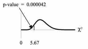
Critical Region
This image shows the graph of the critical region in our example.
Probability statement:
Compare
Make a decision: Since
Conclusion: At a 5% level of significance, from the data, there is sufficient evidence to conclude that a single line causes a lower variation among the waiting times; or, with a single line, the customer waiting times vary less than 7.2 minutes.