A Hypothesis Test for a Single Mean—Standard Deviation Unknown
As an example of a hypothesis test for a single mean, consider the following. Statistics students believe that the mean score on the first statistics test is 65. A statistics instructor thinks the mean score is lower than 65. He randomly samples 10 statistics student scores and obtains the scores [62, 54, 64, 58, 70, 67, 63, 59, 69, 64]. He performs a hypothesis test using a 5% level of significance.
1. State the question: State what we want to determine and what level of significance is important in your decision.
We are asked to test the hypothesis that the mean statistics score,
2. Plan: Based on the above question(s) and the answer to the following questions, decide which test you will be performing. Is the problem about numerical or categorical data? If the data is numerical is the population standard deviation known? Do you have one group or two groups? What type of model is this?
We have univariate, quantitative data. We have a sample of 10 scores. We do not know the population standard deviation. Therefore, we can perform a Student's
3. Hypotheses: State the null and alternative hypotheses in words and then in symbolic form Express the hypothesis to be tested in symbolic form. Write a symbolic expression that must be true when the original claim is false. The null hypothesis is the statement which included the equality. The alternative hypothesis is the statement without the equality.
Null hypothesis in words: The null hypothesis is that the true mean of the statistics exam is equal to 65.
Null hypothesis symbolically:
Alternative hypothesis in words: The alternative is that the true mean statistics score on average is less than 65.
Alternative hypothesis symbolically:
4. The criteria for the inferential test stated above: Think about the assumptions and check the conditions. If your assumptions include the need for particular types of data distribution, construct appropriate graphs or charts.
Randomization Condition: The sample is a random sample.
Independence Assumption: It is reasonable to think that the scores of students are independent in a random sample. There is no reason to think the score of one exam has any bearing on the score of another exam.
10% Condition: We assume the number of statistic students is more than 100, so 10 scores is less than 10% of the population.
Nearly Normal Condition: We should look at a boxplot and histogram for this, shown respectively in and .
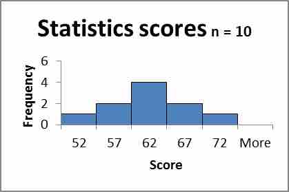
Histogram
This figure shows a histogram for the dataset in our example.
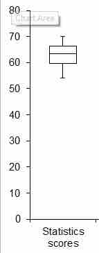
Boxplot
This figure shows a boxplot for the dataset in our example.
Since there are no outliers and the histogram is bell shaped, the condition is satisfied.
Sample Size Condition: Since the distribution of the scores is normal, our sample of 10 scores is large enough.
5. Compute the test statistic:
The conditions are satisfied and σ is unknown, so we will use a hypothesis test for a mean with unknown standard deviation. We need the sample mean, sample standard deviation and Standard Error (SE).
6. Determine the Critical Region(s): Based on your hypotheses, should we perform a left-tailed, right-tailed, or two-sided test?
We will perform a left-tailed test, since we are only concerned with the score being less than 65.
7. Sketch the test statistic and critical region: Look up the probability on the table shown in .
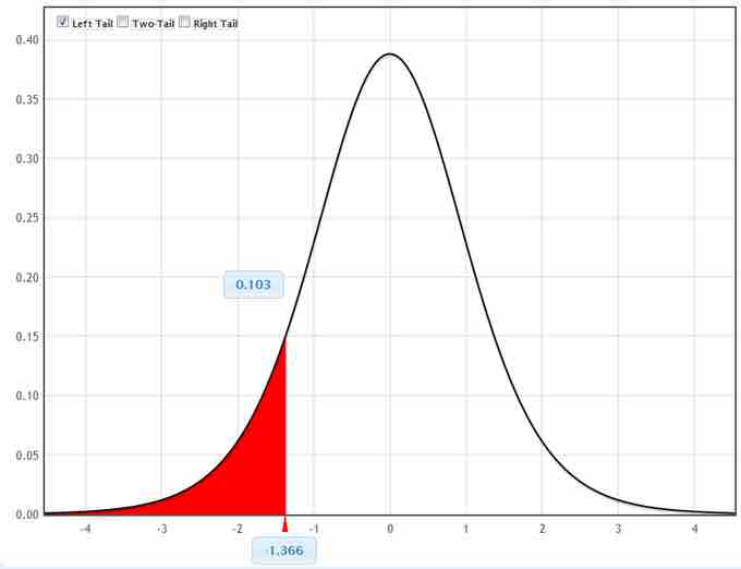
Critical Region
This graph shows the critical region for the test statistic in our example.
8. Determine the
9. State whether you reject or fail to reject the null hypothesis:
Since the probability is greater than than the critical value of 5%, we will fail to reject the null hypothesis.
10. Conclusion: Interpret your result in the proper context, and relate it to the original question.
Since the probability is greater than 5%, this is not considered a rare event and the large probability tells us not to reject the null hypothesis. It is likely that the average statistics score is 65. The