Statistics
Textbooks
Boundless Statistics
Estimation and Hypothesis Testing
Hypothesis Testing: One Sample
Statistics Textbooks Boundless Statistics Estimation and Hypothesis Testing Hypothesis Testing: One Sample
Statistics Textbooks Boundless Statistics Estimation and Hypothesis Testing
Statistics Textbooks Boundless Statistics
Statistics Textbooks
Statistics
Concept Version 6
Created by Boundless

Significance Levels

If a test of significance gives a $p$-value lower than or equal to the significance level, the null hypothesis is rejected at that level.

Learning Objective

  • Outline the process for calculating a $p$-value and recognize its role in measuring the significance of a hypothesis test.


Key Points

    • Significance levels may be used either as a cutoff mark for a $p$-value or as a desired parameter in the test design.
    • To compute a $p$-value from the test statistic, one must simply sum (or integrate over) the probabilities of more extreme events occurring.
    • In some situations, it is convenient to express the complementary statistical significance (so 0.95 instead of 0.05), which corresponds to a quantile of the test statistic.
    • Popular levels of significance are 10% (0.1), 5% (0.05), 1% (0.01), 0.5% (0.005), and 0.1% (0.001).
    • The lower the significance level chosen, the stronger the evidence required.

Terms

  • Student's t-test

    Any statistical hypothesis test in which the test statistic follows a Student's $t$ distribution if the null hypothesis is supported.

  • p-value

    The probability of obtaining a test statistic at least as extreme as the one that was actually observed, assuming that the null hypothesis is true.


Full Text

A fixed number, most often 0.05, is referred to as a significance level or level of significance. Such a number may be used either as a cutoff mark for a $p$-value or as a desired parameter in the test design.

$p$-Value

In brief, the (left-tailed)
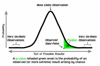
 $p$-value is the quantile of the value of the test statistic, with respect to the sampling distribution under the null hypothesis. The right-tailed $p$-value is one minus the quantile, while the two-tailed $p$-value is twice whichever of these is smaller. Computing a $p$-value requires a null hypothesis, a test statistic (together with deciding if one is doing one-tailed test or a two-tailed test), and data. The key preparatory computation is computing the cumulative distribution function (CDF) of the sampling distribution of the test statistic under the null hypothesis, which may depend on parameters in the null distribution and the number of samples in the data. The test statistic is then computed for the actual data and its quantile is computed by inputting it into the CDF. An example of a $p$-value graph is shown below.

$p$-Value Graph

Example of a $p$-value computation. The vertical coordinate is the probability density of each outcome, computed under the null hypothesis. The $p$-value is the area under the curve past the observed data point.

Hypothesis tests, such as Student's $t$-test, typically produce test statistics whose sampling distributions under the null hypothesis are known. For instance, in the example of flipping a coin, the test statistic is the number of heads produced. This number follows a known binomial distribution if the coin is fair, and so the probability of any particular combination of heads and tails can be computed. To compute a $p$-value from the test statistic, one must simply sum (or integrate over) the probabilities of more extreme events occurring. For commonly used statistical tests, test statistics and their corresponding $p$-values are often tabulated in textbooks and reference works.

Using Significance Levels

Popular levels of significance are 10% (0.1), 5% (0.05), 1% (0.01), 0.5% (0.005), and 0.1% (0.001). If a test of significance gives a $p$-value lower than or equal to the significance level, the null hypothesis is rejected at that level. Such results are informally referred to as statistically significant (at the $p=0.05$ level, etc.). For example, if someone argues that "there's only one chance in a thousand this could have happened by coincidence", a 0.001 level of statistical significance is being stated. The lower the significance level chosen, the stronger the evidence required. The choice of significance level is somewhat arbitrary, but for many applications, a level of 5% is chosen by convention.

In some situations, it is convenient to express the complementary statistical significance (so 0.95 instead of 0.05), which corresponds to a quantile of the test statistic. In general, when interpreting a stated significance, one must be careful to make precise note of what is being tested statistically.

Different levels of cutoff trade off countervailing effects. Lower levels – such as 0.01 instead of 0.05 – are stricter and increase confidence in the determination of significance, but they run an increased risk of failing to reject a false null hypothesis. Evaluation of a given $p$-value of data requires a degree of judgment; and rather than a strict cutoff, one may instead simply consider lower $p$-values as more significant.

[ edit ]
Edit this content
Prev Concept
Type I and Type II Errors
Directional Hypotheses and One-Tailed Tests
Next Concept
Subjects
  • Accounting
  • Algebra
  • Art History
  • Biology
  • Business
  • Calculus
  • Chemistry
  • Communications
  • Economics
  • Finance
  • Management
  • Marketing
  • Microbiology
  • Physics
  • Physiology
  • Political Science
  • Psychology
  • Sociology
  • Statistics
  • U.S. History
  • World History
  • Writing

Except where noted, content and user contributions on this site are licensed under CC BY-SA 4.0 with attribution required.