Damped Harmonic Motion

The Physical Situation

The simple harmonic oscillator describes many physical systems throughout the world, but early studies of physics usually only consider ideal situations that do not involve friction. In the real world, however, frictional forces - such as air resistance - will slow, or dampen, the motion of an object. Sometimes, these dampening forces are strong enough to return an object to equilibrium over time .

Damped Harmonic Motion

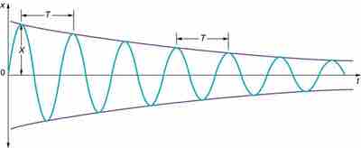
Illustrating the position against time of our object moving in simple harmonic motion. We see that for small damping, the amplitude of our motion slowly decreases over time.

The simplest and most commonly seen case occurs when the frictional force is proportional to an object's velocity. Note that other cases exist which may lead to nonlinear equations which go beyond the scope of this example.

Consider an object of mass m attached to a spring of constant k. Let the damping force be proportional to the mass' velocity by a proportionality constant, b, called the vicious damping coefficient. We can describe this situation using Newton's second law, which leads to a second order, linear, homogeneous, ordinary differential equation. We simply add a term describing the damping force to our already familiar equation describing a simple harmonic oscillator to describe the general case of damped harmonic motion.

$\begin{array}{lcl} F_{net}&=&m \frac{d^{2}x}{dt^2} + b\frac{dx}{dt} + kx = 0 \\ &=& \frac{d^2x}{dt^2} + \frac{b}{m}\frac{dx}{dt} + \frac{k}{m}x = 0 \\ &= &\frac{d^2x}{dt^2} + \gamma \frac{dx}{dt} + \omega_0^2 x = 0 \\ \end{array} \\ \omega_0^2 = \frac{k}{m}, \gamma = \frac{b}{m}$

This notation uses $\frac{d^2x}{dt^2}$, the acceleration of our object, $\frac{dx}{dt}$, the velocity of our object, $\omega_0$, undamped angular frequency of oscillation, and ɣ, which we can call the damping ratio.

Solving the Differential Equation; Interpreting Results

We solve this differential equation for our equation of motion of the system, x(t). We assume a solution in the form of an exponential, where a is a constant value which we will solve for.

$x(t) = e^{at}$

Plugging this into the differential equation we find that there are three results for a, which will dictate the motion of our system. We can solve for a by using the quadratic equation.

$\begin{array}{lcl} F_{net}&=&a^{2} x + \gamma a x + \omega_0^2 x = 0 \\ &=& a^{2} + \gamma a + \omega_0^2 = 0 \\ \end{array}$

$a = \frac{\gamma \pm \sqrt{\gamma^2 - 4 \omega_0^2}}{2}$

The physical situation has three possible results depending on the value of a, which depends on the value of what is under our radical. This expression can be positive, negative, or equal to zero which will result in overdamping, underdamping, and critical damping, respectively.

$\gamma^2 > 4\omega_0^2$ is the Over Damped case. In this case, the system returns to equilibrium by exponentially decaying towards zero. The system will not pass the equilibrium position more than once.

$\gamma^2 < 4\omega_0^2$ is the Under Damped case. In this case, the system oscillates as it slowly returns to equilibrium and the amplitude decreases over time. Figure 1 depicts an underdamped case.

$\gamma^2 = 4\omega_0^2$ is theCritically Damped case. In this case, the system returns to equilibrium very quickly without oscillating and without passing the equilibrium position at all.