Calculus
Textbooks
Boundless Calculus
Inverse Functions and Advanced Integration
Techniques of Integration
Calculus Textbooks Boundless Calculus Inverse Functions and Advanced Integration Techniques of Integration
Calculus Textbooks Boundless Calculus Inverse Functions and Advanced Integration
Calculus Textbooks Boundless Calculus
Calculus Textbooks
Calculus
Concept Version 7
Created by Boundless

Numerical Integration

Numerical integration constitutes a broad family of algorithms for calculating the numerical value of a definite integral.

Learning Objective

  • Solve definite integrals


Key Points

    • The basic problem considered by numerical integration is to compute an approximate solution to a definite integral: $\int_a^b\! f(x)\, dx$.
    • There are several reasons for carrying out numerical integration. It could be due to the specific nature of the function (to be integrated) or its antiderivatives.
    • A large class of quadrature rules can be derived by constructing interpolating functions which are easy to integrate. Typically these interpolating functions are polynomials. Midpoint method and trapezoidal method are simple examples.

Terms

  • trapezoidal

    in the shape of a trapezoid, or having some faces which have one pair of parallel sides

  • antiderivative

    an indefinite integral


Full Text

Numerical integration constitutes a broad family of algorithms for calculating the numerical value of a definite integral, and, by extension, the term is also sometimes used to describe the numerical solution of differential equations. This article focuses on calculation of definite integrals. The term numerical quadrature (often abbreviated to quadrature) is more or less a synonym for numerical integration, especially as applied to one-dimensional integrals. Numerical integration over more than one dimension is sometimes described as cubature, although the meaning of quadrature is understood for higher dimensional integration as well.

The basic problem considered by numerical integration is to compute an approximate solution to a definite integral: 

$\displaystyle{\int_a^b\! f(x)\, dx}$

If $f(x)$ is a smooth well-behaved function, integrated over a small number of dimensions and the limits of integration are bounded, there are many methods of approximating the integral with arbitrary precision.

Reasons for numerical integration

  1. There are several reasons for carrying out numerical integration. The integrand $f(x)$ may be known only at certain points, such as when obtained by sampling. Some embedded systems and other computer applications may need numerical integration for this reason.
  2. A formula for the integrand may be known, but it may be difficult or impossible to find an antiderivative which is an elementary function. An example of such an integrand $f(x)=\exp(-x^2)$, the antiderivative of which (the error function, times a constant) cannot be written in elementary form.
  3. It may be possible to find an antiderivative symbolically, but it may be easier to compute a numerical approximation than to compute the antiderivative. That may be the case if the antiderivative is given as an infinite series or product, or if its evaluation requires a special function which is not available.

Methods for One-Dimensional Integrals

A large class of quadrature rules can be derived by constructing interpolating functions which are easy to integrate. Typically these interpolating functions are polynomials. The simplest method of this type is to let the interpolating function be a constant function (a polynomial of degree zero) which passes through the point
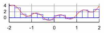
 $\left(\frac{(a+b)}{2}, f\left(\frac{(a+b)}{2}\right)\right)$. This is called the midpoint rule or rectangle rule: 

$\displaystyle{\int_a^b f(x)\,dx \approx (b-a) \, f\left(\frac{a+b}{2}\right)}$

Rectangle Rule

Illustration of the rectangle rule.

The interpolating function may be an affine function (a polynomial of degree 1) which passes through the points
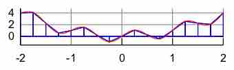
 $(a, f(a))$ and $(b, f(b))$. This is called the trapezoidal rule.

Trapezoidal Rule

Illustration of the trapezoidal rule.

For either one of these rules, we can make a more accurate approximation by breaking up the interval $[a, b]$ into some number $n$ of subintervals, computing an approximation for each subinterval, then adding up all the results. This is called a composite rule, extended rule, or iterated rule. For example, the composite trapezoidal rule can be stated as 

$\displaystyle{\int_a^b f(x)\,dx \approx \frac{b-a}{n} \left( {f(a) \over 2} + \sum_{k=1}^{n-1} \left( f \left( a+k \frac{b-a}{n} \right) \right) + {f(b) \over 2} \right)}$

where the subintervals have the form $[k h, (k+1) h]$, with $h= \frac{(b-a)}{n}$  and $k = 0, 1, 2, \cdots, n−1$.

[ edit ]
Edit this content
Prev Concept
Improper Integrals
Arc Length and Surface Area
Next Concept
Subjects
  • Accounting
  • Algebra
  • Art History
  • Biology
  • Business
  • Calculus
  • Chemistry
  • Communications
  • Economics
  • Finance
  • Management
  • Marketing
  • Microbiology
  • Physics
  • Physiology
  • Political Science
  • Psychology
  • Sociology
  • Statistics
  • U.S. History
  • World History
  • Writing

Except where noted, content and user contributions on this site are licensed under CC BY-SA 4.0 with attribution required.