Calculus
Textbooks
Boundless Calculus
Derivatives and Integrals
Integrals
Calculus Textbooks Boundless Calculus Derivatives and Integrals Integrals
Calculus Textbooks Boundless Calculus Derivatives and Integrals
Calculus Textbooks Boundless Calculus
Calculus Textbooks
Calculus
Concept Version 9
Created by Boundless

Numerical Integration

Numerical integration is a method of approximating the value of a definite integral.

Learning Objective

  • Solve for the definite integral of a continuous function over a closed interval


Key Points

    • Numerical methods of approximation are useful when the integral is difficult to solve by hand.
    • Some methods of numerical integration include the rectangle rule and the trapezoidal rule.
    • Since computers cannot solve integrals by hand and are very fast at arithmetic, they use numerical methods to solve integrals.

Terms

  • approximation

    An imprecise solution or result that is adequate for a defined purpose.

  • definite integral

    the integral of a function between an upper and lower limit


Full Text

Given a function $f$ of a real variable $x$ and an interval of the real line, the definite integral $\int_{a}^{b}f(x)dx $ is defined informally to be the area of the region in the $xy$-plane bound by the graph of $f$, the $x$-axis, and the vertical lines $x=a$ and $x=b$, such that the area above the $x$-axis adds to the total, and that the area below the $x$-axis subtracts from the total. These integrals are termed "definite integrals."

Definite Integral

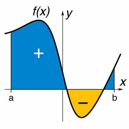
A definite integral of a function can be represented as the signed area of the region bounded by its graph.

Numerical integration constitutes a broad family of algorithms for calculating the numerical value of a definite integral.

There are several reasons for carrying out numerical integration.

The integrand $f(x)$ may be known only at certain points, such as obtained by sampling. Some embedded systems and other computer applications may need numerical integration for this reason.

A formula for the integrand may be known, but it may be difficult or impossible to find an antiderivative which is an elementary function. An example of such an integrand is $f(x) = \exp(x^2)$, the antiderivative of which (the error function, times a constant) cannot be written in elementary form. It may be possible to find an antiderivative symbolically, but it may be easier to compute a numerical approximation than to compute the antiderivative. That may be the case if the antiderivative is given as an infinite series or product, or if its evaluation requires a special function which is not available.

Numerical integration methods can generally be described as combining evaluations of the integrand to get an approximation to the integral.

The integrand is evaluated at a finite set of points called integration points and a weighted sum of these values is used to approximate the integral. The integration points and weights depend on the specific method used and the accuracy required from the approximation. An important part of the analysis of any numerical integration method is to study the behavior of the approximation error as a function of the number of integrand evaluations. A method which yields a small error for a small number of evaluations is usually considered superior. Reducing the number of evaluations of the integrand reduces the number of arithmetic operations involved, and therefore reduces the total round-off error. Also, each evaluation takes time, and the integrand may be arbitrarily complicated. A 'brute force' kind of numerical integration can be done, if the integrand is reasonably well-behaved (i.e. piecewise continuous and of bounded variation), by evaluating the integrand with very small increments.

The simplest method to numerically solve integrals is to use the midpoint or rectangle rule. Draw rectangles which pass through the following point:

$\displaystyle{\left ( \frac{(a+b)}{2}, f \left ( \frac{(a+b)}{2} \right ) \right )}$

The way to do this is as follows:

$\displaystyle{∫_b^af(x)dx \approx (b−a)f \left ( \frac{a+b}{2} \right ) }$

The area can then be approximated by adding up the areas of the rectangles. Notice that the smaller the rectangles are made, the more accurate the approximation.
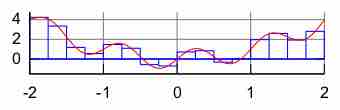
Rectangle Rule

Illustration of the rectangle rule of numerical integration. The value of $f(x)$ is taken to be constant around a point and the integral is calculated by adding up the areas of the rectangles.

The trapezoidal rule is a more accurate method of numerical integration. Instead of taking
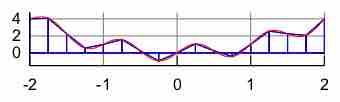
 $f(x)$ to be a constant around a chosen $x$, $f(x)$ is approximated as having a constant slope around $x$, where the slope is the average between the chosen points.

$\begin{aligned}\int_{a}^{b} f(x) dx &\approx(b - a) f(a) + f(b) 2\int_a^b f(x)dx\\ & \approx (b-a) \frac{f(a) + f(b)}{2}\end{aligned}$

Trapezoidal Rule

Illustration of the trapezoidal rule.

For either one of these rules, we can make a more accurate approximation by breaking up the interval $[a, b]$ into some number $n$ of subintervals, computing an approximation for each subinterval, then adding up all the results. This is called a composite rule, extended rule, or iterated rule. For example, the composite trapezoidal rule can be stated as:

$\displaystyle{\int_a^b f(x)\,dx \approx \frac{b-a}{n} \left( {f(a) \over 2} + \sum_{k=1}^{n-1} \left( f \left( a+k \frac{b-a}{n} \right) \right) + {f(b) \over 2} \right)}$

where the subintervals have the form $[k h, (k+1) h]$, with $h = \frac{(b−a)}{n}$ and $k = 0, 1, 2, \cdots , n−1$.

Since computers are able to do many arithmetic operations in a small amount of time, they use numerical integration to approximate the values of integrals rather than solving them the way a person would.

[ edit ]
Edit this content
Prev Concept
Further Transcendental Functions
Area Between Curves
Next Concept
Subjects
  • Accounting
  • Algebra
  • Art History
  • Biology
  • Business
  • Calculus
  • Chemistry
  • Communications
  • Economics
  • Finance
  • Management
  • Marketing
  • Microbiology
  • Physics
  • Physiology
  • Political Science
  • Psychology
  • Sociology
  • Statistics
  • U.S. History
  • World History
  • Writing

Except where noted, content and user contributions on this site are licensed under CC BY-SA 4.0 with attribution required.