Second-Order Linear Equations

Linear differential equations are of the form $Ly = f$, where the differential operator $L$ is a linear operator, $y$ is the unknown function (such as a function of time $y(t)$), and the right hand side $f$ is a given function of the same nature as $y$ (called the source term). For a function dependent on time, we may write the equation more expressly as $L y(t) = f(t)$ and, even more precisely, by bracketing $L [y(t)] = f(t)$.

The linear operator $L$ may be considered to be of the form:

$\displaystyle{L_n(y) \equiv \frac{d^n y}{dt^n} + A_1(t)\frac{d^{n-1}y}{dt^{n-1}} + \cdots + A_{n-1}(t)\frac{dy}{dt} + A_n(t)y}$

The linearity condition on $L$ rules out operations such as taking the square of the derivative of $y$, but permits, for example, taking the second derivative of $y$. It is convenient to rewrite this equation in an operator form: 

$\displaystyle{L_n(y) \equiv \left[\,D^n + A_{1}(t)D^{n-1} + \cdots + A_{n-1}(t) D + A_n(t)\right] y}$

where $D$ is the differential operator $\frac{d}{dt}$ (i.e. $Dy = y'$, $D^2y = y''$, $\cdots$) that is involved.

Second-Order Linear Differential Equations

A second-order linear differential equation has the form: 

$\displaystyle{\frac{d^2 y}{dt^2} + A_1(t)\frac{dy}{dt} + A_2(t)y = f(t)}$ 

where $A_1(t)$, $A_2(t)$, and $f(t)$ are continuous functions. When $f(t)=0$, the equations are called homogeneous second-order linear differential equations. (Otherwise, the equations are called nonhomogeneous equations.)

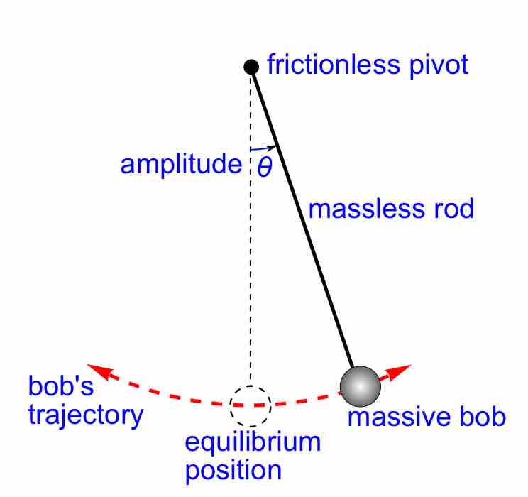
Simple Pendulum

A simple pendulum, under the conditions of no damping and small amplitude, is described by a equation of motion which is a second-order linear differential equation.