In mathematical optimization, the method of Lagrange multipliers (named after Joseph Louis Lagrange) is a strategy for finding the local maxima and minima of a function subject to equality constraints.
For instance, consider the following optimization problem: Maximize
where the
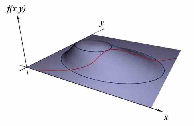
Maximizing f(x,y)
Find x and y to maximize f(x,y) subject to a constraint (shown in red) g(x,y)=c.
Introduction
One of the most common problems in calculus is that of finding maxima or minima (in general, "extrema") of a function, but it is often difficult to find a closed form for the function being extremized. Such difficulties often arise when one wishes to maximize or minimize a function subject to fixed outside conditions or constraints. The method of Lagrange multipliers is a powerful tool for solving this class of problems without the need to explicitly solve the conditions and use them to eliminate extra variables.
Consider the two-dimensional problem introduced above. Maximize
The contour lines of
and
The constant is required because, although the two gradient vectors are parallel, the magnitudes of the gradient vectors are generally not equal. Note that
To incorporate these conditions into one equation, we introduce an auxiliary function,
Where the Lagrange multiplier
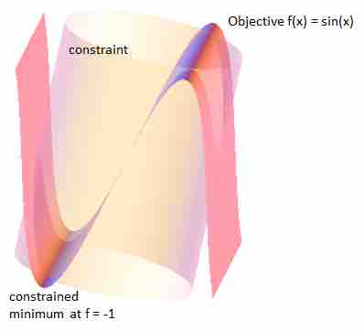
Minimize