The Standard Normal Curve

If the mean ($\mu$) and standard deviation ($\sigma$) of a normal distribution are 0 and 1, respectively, then we say that the random variable follows a standard normal distribution. This type of random variable is often denoted by $Z$, instead of $X$.

The area above the $x$-axis and under the curve must equal one, with the area under the curve representing the probability. For example, $P(-2<X<2)$ is the area under the curve between $x=-2$ and $x=2$. Since the standard deviation is 1, this represents the probability that a normal distribution is between 2 standard deviations away from the mean. From the empirical rule, we know that this value is 0.95.

Standardization

Unfortunately, in most cases in which the normal distribution plays a role, the mean is not 0 and the standard deviation is not 1. Luckily, one can transform any normal distribution with a certain mean $\mu$ and standard deviation $\sigma$ into a standard normal distribution, by the $z$-score conversion formula:

$\displaystyle z=\frac { x-\mu }{ \sigma }$

Therefore, a $z$-score is the standardized value of observation $x$ from a distribution that has mean $\mu$ and standard deviation $\sigma$ (how many standard deviations you are away from zero). The $z$-score gets its name because of the denomination of the standard normal distribution as the "$Z$" distribution. It can be said to provide an assessment of how off-target a process is operating.

A key point is that calculating $z$ requires the population mean and the population standard deviation, not the sample mean or sample deviation. It requires knowing the population parameters, not the statistics of a sample drawn from the population of interest. However, knowing the true standard deviation of a population is often unrealistic except in cases such as standardized testing, where the entire population is measured. In cases where it is impossible to measure every member of a population, the standard deviation may be estimated using a random sample.

Example

Assuming that the height of women in the US is normally distributed with a mean of 64 inches and a standard deviation of 2.5 inches, find the following:

1. The probability that a randomly selected woman is taller than 70.4 inches (5 foot 10.4 inches).
2. The probability that a randomly selected woman is between 60.3 and 65 inches tall.

Part one: Since the height of women follows a normal distribution but not a standard normal, we first need to standardize. Since $x=70.4 \ \text{inches}$, $\mu=64 \ \text{inches}$ and $\sigma = 2.5 \ \text{inches}$, we need to calculate $z$:

$\displaystyle z=\frac { 70.4-64 }{ 2.5 } =\frac { 6.4 }{ 2.5 } =2.56$

Therefore, the probability $P(X>70.4)$ is equal to $P(Z>2.56)$, where $X$ is the normally distributed height with mean $\mu=64 \ \text{inches}$ and standard deviation $\sigma = 2.5 \ \text{inches}$ ($\{X \sim N(64, 2.5)\}$, for short), and $Z$ is a standard normal distribution $\{Z \sim N(0, 1)\}$.

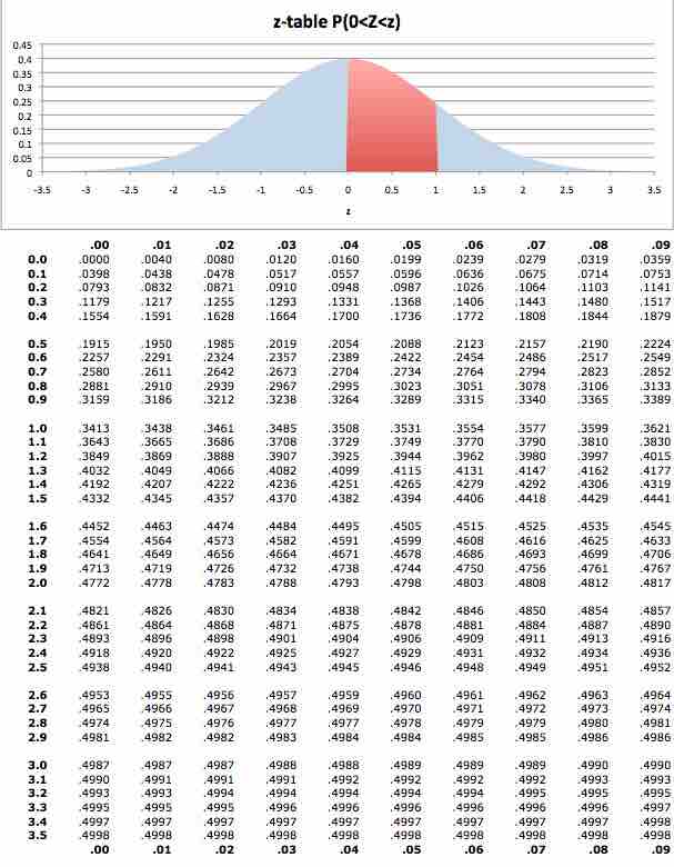
The next step requires that we use what is known as the $z$-score table to calculate probabilities for the standard normal distribution. This table can be seen below.

$z$-table

The $z$-score table is used to calculate probabilities for the standard normal distribution.

From the table, we learn that:

$P(X>70.4)=P(Z>2.56)$

$\qquad \qquad \ \ \ =0.5-0.4948$

$\qquad \qquad \ \ \ = 0.0012$

Part two: For the second problem we have two values of $x$ to standarize: $x_1 = 60.3$and $x_2 = 65$. Standardizing these values we obtain:

$z_1 = -1.48$ and $z_2 = 0.40$.

Notice that the first value is negative, which means that it is below the mean. Therefore:

$P(60.3<X<65) = P(-1.48<Z<0.40)$

$\qquad \qquad \qquad \quad = P(Z<0.40)-P(Z<-1.48)$

$\qquad \qquad \qquad \quad = (0.5+0.1554)-(0.5-0694)$

$\qquad \qquad \qquad \quad = 0.6554-0.0694$

$\qquad \qquad \qquad \quad = 0.5860$