Statistics
Textbooks
Boundless Statistics
Visualizing Data
The Histogram
Statistics Textbooks Boundless Statistics Visualizing Data The Histogram
Statistics Textbooks Boundless Statistics Visualizing Data
Statistics Textbooks Boundless Statistics
Statistics Textbooks
Statistics
Concept Version 8
Created by Boundless

The Density Scale

Density estimation is the construction of an estimate based on observed data of an unobservable, underlying probability density function.

Learning Objective

  • Describe how density estimation is used as a tool in the construction of a histogram.


Key Points

    • The unobservable density function is thought of as the density according to which a large population is distributed. The data are usually thought of as a random sample from that population.
    • A probability density function, or density of a continuous random variable, is a function that describes the relative likelihood for a random variable to take on a given value.
    • Kernel density estimates are closely related to histograms, but can be endowed with properties such as smoothness or continuity by using a suitable kernel.

Terms

  • quartile

    any of the three points that divide an ordered distribution into four parts, each containing a quarter of the population

  • density

    the probability that an event will occur, as a function of some observed variable

  • interquartile range

    The difference between the first and third quartiles; a robust measure of sample dispersion.


Full Text

Density Estimation

Histograms are used to plot the density of data, and are often a useful tool for density estimation. Density estimation is the construction of an estimate based on observed data of an unobservable, underlying probability density function. The unobservable density function is thought of as the density according to which a large population is distributed. The data are usually thought of as a random sample from that population.

A probability density function, or density of a continuous random variable, is a function that describes the relative likelihood for this random variable to take on a given value. The probability for the random variable to fall within a particular region is given by the integral of this variable's density over the region .

Boxplot Versus Probability Density Function

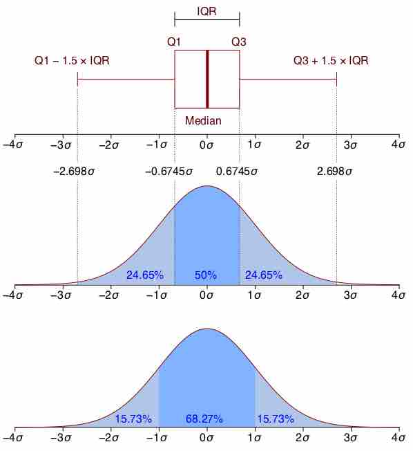
This image shows a boxplot and probability density function of a normal distribution.

The above image depicts a probability density function graph against a box plot. A box plot is a convenient way of graphically depicting groups of numerical data through their quartiles. The spacings between the different parts of the box help indicate the degree of dispersion (spread) and skewness in the data and to identify outliers. In addition to the points themselves, box plots allow one to visually estimate the interquartile range.

A range of data clustering techniques are used as approaches to density estimation, with the most basic form being a rescaled histogram.

Kernel Density Estimation

Kernel density estimates are closely related to histograms, but can be endowed with properties such as smoothness or continuity by using a suitable kernel. To see this, we compare the construction of histogram and kernel density estimators using these 6 data points:

$x_1 = -2.1$, $x_2 = -1.3$, $x_3 = -0.4$, $x_4=1.9$, $x_5=5.1$, $x_6=6.2$

For the histogram, first the horizontal axis is divided into sub-intervals, or bins, which cover the range of the data. In this case, we have 6 bins, each having a width of 2. Whenever a data point falls inside this interval, we place a box of height $\frac{1}{12}$. If more than one data point falls inside the same bin, we stack the boxes on top of each other .

Histogram Versus Kernel Density Estimation

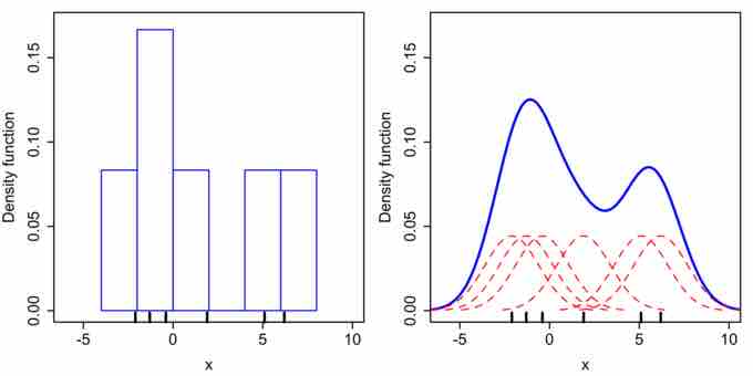
Comparison of the histogram (left) and kernel density estimate (right) constructed using the same data. The 6 individual kernels are the red dashed curves, the kernel density estimate the blue curves. The data points are the rug plot on the horizontal axis.

For the kernel density estimate, we place a normal kernel with variance 2.25 (indicated by the red dashed lines) on each of the data points $x_i$. The kernels are summed to make the kernel density estimate (the solid blue curve). Kernel density estimates converge faster to the true underlying density for continuous random variables thus accounting for their smoothness compared to the discreteness of the histogram.

[ edit ]
Edit this content
Prev Concept
Recognizing and Using a Histogram
Types of Variables
Next Concept
Subjects
  • Accounting
  • Algebra
  • Art History
  • Biology
  • Business
  • Calculus
  • Chemistry
  • Communications
  • Economics
  • Finance
  • Management
  • Marketing
  • Microbiology
  • Physics
  • Physiology
  • Political Science
  • Psychology
  • Sociology
  • Statistics
  • U.S. History
  • World History
  • Writing

Except where noted, content and user contributions on this site are licensed under CC BY-SA 4.0 with attribution required.