To construct a histogram, one must first decide how many bars or intervals (also called classes) are needed to represent the data. Many histograms consist of between 5 and 15 bars, or classes. One must choose a starting point for the first interval, which must be less than the smallest data value. A convenient starting point is a lower value carried out to one more decimal place than the value with the most decimal places.
For example, if the value with the most decimal places is 6.1, and this is the smallest value, a convenient starting point is 6.05 (
Consider the following data, which are the heights (in inches to the nearest half inch) of 100 male semiprofessional soccer players. The heights are continuous data since height is measured.
60; 60.5; 61; 61; 61.5; 63.5; 63.5; 63.5; 64; 64; 64; 64; 64; 64; 64; 64.5; 64.5; 64.5; 64.5; 64.5; 64.5; 64.5; 64.5; 66; 66; 66; 66; 66; 66; 66; 66; 66; 66; 66.5; 66.5; 66.5; 66.5; 66.5; 66.5; 66.5; 66.5; 66.5; 66.5; 66.5; 67; 67; 67; 67; 67; 67; 67; 67; 67; 67; 67; 67; 67.5; 67.5; 67.5; 67.5; 67.5; 67.5; 67.5; 68; 68; 69; 69; 69; 69; 69; 69; 69; 69; 69; 69; 69.5; 69.5; 69.5; 69.5; 69.5; 70; 70; 70; 70; 70; 70; 70.5; 70.5; 70.5; 71; 71; 71; 72; 72; 72; 72.5; 72.5; 73; 73.5; 74
The smallest data value is 60. Since the data with the most decimal places has one decimal (for instance, 61.5), we want our starting point to have two decimal places. Since the numbers 0.5, 0.05, 0.005, and so on are convenient numbers, use 0.05 and subtract it from 60, the smallest value, for the convenient starting point. The starting point, then, is 59.95.
The largest value is 74.
Next, calculate the width of each bar or class interval. To calculate this width, subtract the starting point from the ending value and divide by the number of bars (you must choose the number of bars you desire). Note that there is no "best" number of bars, and different bar sizes can reveal different features of the data. Some theoreticians have attempted to determine an optimal number of bars, but these methods generally make strong assumptions about the shape of the distribution. Depending on the actual data distribution and the goals of the analysis, different bar widths may be appropriate, so experimentation is usually needed to determine an appropriate width.
Suppose, in our example, we choose 8 bars. The bar width will be as follows:
We will round up to 2 and make each bar or class interval 2 units wide. Rounding up to 2 is one way to prevent a value from falling on a boundary. The boundaries are:
59.95, 61.95, 63.95, 65.95, 67.95, 69.95, 71.95, 73.95, 75.95
So that there are 2 units between each boundary.
The heights 60 through 61.5 inches are in the interval 59.95 - 61.95. The heights that are 63.5 are in the interval 61.95 - 63.95. The heights that are 64 through 64.5 are in the interval 63.95 - 65.95. The heights 66 through 67.5 are in the interval 65.95 - 67.95. The heights 68 through 69.5 are in the interval 67.95 - 69.95. The heights 70 through 71 are in the interval 69.95 - 71.95. The heights 72 through 73.5 are in the interval 71.95 - 73.95. The height 74 is in the interval 73.95 - 75.95.
displays the heights on the x-axis and relative frequency on the y-axis.
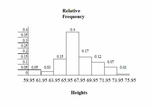
Histogram Example
This histogram depicts the relative frequency of heights for 100 semiprofessional soccer players. Note the roughly normal distribution, with the center of the curve around 66 inches.