Statistics
Textbooks
Boundless Statistics
Sampling
Sampling Distributions
Statistics Textbooks Boundless Statistics Sampling Sampling Distributions
Statistics Textbooks Boundless Statistics Sampling
Statistics Textbooks Boundless Statistics
Statistics Textbooks
Statistics
Concept Version 8
Created by Boundless

Sampling Distributions and the Central Limit Theorem

The central limit theorem for sample means states that as larger samples are drawn, the sample means form their own normal distribution.

Learning Objective

  • Illustrate that as the sample size gets larger, the sampling distribution approaches normality


Key Points

    • The normal distribution has the same mean as the original distribution and a variance that equals the original variance divided by $n$, the sample size.
    • $n$ is the number of values that are averaged together not the number of times the experiment is done.
    • The usefulness of the theorem is that the sampling distribution approaches normality regardless of the shape of the population distribution.

Terms

  • central limit theorem

    The theorem that states: If the sum of independent identically distributed random variables has a finite variance, then it will be (approximately) normally distributed.

  • sampling distribution

    The probability distribution of a given statistic based on a random sample.


Example

    • Imagine rolling a large number of identical, unbiased dice. The distribution of the sum (or average) of the rolled numbers will be well approximated by a normal distribution. Since real-world quantities are often the balanced sum of many unobserved random events, the central limit theorem also provides a partial explanation for the prevalence of the normal probability distribution. It also justifies the approximation of large-sample statistics to the normal distribution in controlled experiments.

Full Text

The central limit theorem states that, given certain conditions, the mean of a sufficiently large number of independent random variables, each with a well-defined mean and well-defined variance, will be (approximately) normally distributed. The central limit theorem has a number of variants. In its common form, the random variables must be identically distributed. In variants, convergence of the mean to the normal distribution also occurs for non-identical distributions, given that they comply with certain conditions.

The central limit theorem for sample means specifically says that if you keep drawing larger and larger samples (like rolling 1, 2, 5, and, finally, 10 dice) and calculating their means the sample means form their own normal distribution (the sampling distribution). The normal distribution has the same mean as the original distribution and a variance that equals the original variance divided by $n$, the sample size. $n$ is the number of values that are averaged together not the number of times the experiment is done.

Classical Central Limit Theorem

Consider a sequence of independent and identically distributed random variables drawn from distributions of expected values given by $\mu$ and finite variances given by $\sigma^2$. Suppose we are interested in the sample average of these random variables. By the law of large numbers, the sample averages converge in probability and almost surely to the expected value $\mu$ as $n \rightarrow \infty$. The classical central limit theorem describes the size and the distributional form of the stochastic fluctuations around the deterministic number $\mu$ during this convergence. More precisely, it states that as $n$ gets larger, the distribution of the difference between the sample average $S_n$ and its limit $\mu$ approximates the normal distribution with mean 0 and variance $\sigma^2$. For large enough $n$, the distribution of $S_n$ is close to the normal distribution with mean $\mu$ and variance

$\displaystyle \frac { { \sigma }^{ 2 } }{ n }$

The upshot is that the sampling distribution of the mean approaches a normal distribution as $n$, the sample size, increases. The usefulness of the theorem is that the sampling distribution approaches normality regardless of the shape of the population distribution.

Empirical Central Limit Theorem

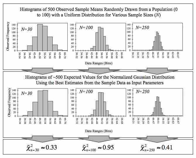
This figure demonstrates the central limit theorem. The sample means are generated using a random number generator, which draws numbers between 1 and 100 from a uniform probability distribution. It illustrates that increasing sample sizes result in the 500 measured sample means being more closely distributed about the population mean (50 in this case).

[ edit ]
Edit this content
Prev Concept
Shapes of Sampling Distributions
Expected Value and Standard Error
Next Concept
Subjects
  • Accounting
  • Algebra
  • Art History
  • Biology
  • Business
  • Calculus
  • Chemistry
  • Communications
  • Economics
  • Finance
  • Management
  • Marketing
  • Microbiology
  • Physics
  • Physiology
  • Political Science
  • Psychology
  • Sociology
  • Statistics
  • U.S. History
  • World History
  • Writing

Except where noted, content and user contributions on this site are licensed under CC BY-SA 4.0 with attribution required.