Using the Normal Curve

$z$-Value

The functional form for a normal distribution is a bit complicated. It can also be difficult to compare two variables if their mean and or standard deviations are different. For example, heights in centimeters and weights in kilograms, even if both variables can be described by a normal distribution. To get around both of these conflicts, we can define a new variable:

$\displaystyle z=\frac{x-\mu }{\sigma }$ 

This variable gives a measure of how far the variable is from the mean ($x-\mu$), then "normalizes" it by dividing by the standard deviation ($\sigma$). This new variable gives us a way of comparing different variables. The $z$-value tells us how many standard deviations, or "how many sigmas", the variable is from its respective mean.

Areas Under the Curve

To calculate the probability that a variable is within a range, we have to find the area under the curve. Normally, this would mean we'd need to use calculus. However, statisticians have figured out an easier method, using tables, that can typically be found in your textbook or even on your calculator.

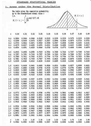
Standard Normal Table

This table can be used to find the cumulative probability up to the standardized normal value $z$.

These tables can be a bit intimidating, but you simply need to know how to read them. The leftmost column tells you how many sigmas above the the mean to one decimal place (the tenths place).The top row gives the second decimal place (the hundredths).The intersection of a row and column gives the probability.

For example, if we want to know the probability that a variable is no more than 0.51 sigmas above the mean, $P(z<0.51)$, we look at the 6^th row down (corresponding to 0.5) and the 2^nd column (corresponding to 0.01). The intersection of the 6^th row and 2^nd column is 0.6950, which tells us that there is a 69.50% percent chance that a variable is less than 0.51 sigmas (or standard deviations) above the mean.

A common mistake is to look up a $z$-value in the table and simply report the corresponding entry, regardless of whether the problem asks for the area to the left or to the right of the $z$-value. The table only gives the probabilities to the left of the $z$-value. Since the total area under the curve is 1, all we need to do is subtract the value found in the table from 1. For example, if we wanted to find out the probability that a variable is more than 0.51 sigmas above the mean, $P(z>0.51)$, we just need to calculate $1-P(z<0.51) = 1-0.6950 = 0.3050$, or 30.5%.

There is another note of caution to take into consideration when using the table: The table provided only gives values for positive $z$-values, which correspond to values above the mean. What if we wished instead to find out the probability that a value falls below a $z$-value of $-0.51$, or 0.51 standard deviations below the mean? We must remember that the standard normal curve is symmetrical , meaning that $P(z<-0.51) = P(z>0.51)$, which we calculated above to be 30.5%.

Symmetrical Normal Curve

This images shows the symmetry of the normal curve. In this case, P(z2.01).

We may even wish to find the probability that a variable is between two z-values, such as between 0.50 and 1.50, or $P(0.50)$.

68-95-99.7 Rule

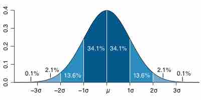
Although we can always use the $z$-score table to find probabilities, the 68-95-99.7 rule helps for quick calculations. In a normal distribution, approximately 68% of values fall within one standard deviation of the mean, approximately 95% of values fall with two standard deviations of the mean, and approximately 99.7% of values fall within three standard deviations of the mean.

68-95-99.7 Rule

Dark blue is less than one standard deviation away from the mean. For the normal distribution, this accounts for about 68% of the set, while two standard deviations from the mean (medium and dark blue) account for about 95%, and three standard deviations (light, medium, and dark blue) account for about 99.7%.