The multiple comparisons problem occurs when one considers a set of statistical inferences simultaneously or infers a subset of parameters selected based on the observed values. Errors in inference, including confidence intervals that fail to include their corresponding population parameters or hypothesis tests that incorrectly reject the null hypothesis, are more likely to occur when one considers the set as a whole. Several statistical techniques have been developed to prevent this, allowing direct comparison of means significance levels for single and multiple comparisons. These techniques generally require a stronger level of observed evidence in order for an individual comparison to be deemed "significant," so as to compensate for the number of inferences being made.
The Problem
When researching, we typically refer to comparisons of two groups, such as a treatment group and a control group. "Multiple comparisons" arise when a statistical analysis encompasses a number of formal comparisons, with the presumption that attention will focus on the strongest differences among all comparisons that are made. Failure to compensate for multiple comparisons can have important real-world consequences
As the number of comparisons increases, it becomes more likely that the groups being compared will appear to differ in terms of at least one attribute. Our confidence that a result will generalize to independent data should generally be weaker if it is observed as part of an analysis that involves multiple comparisons, rather than an analysis that involves only a single comparison.
For example, if one test is performed at the 5% level, there is only a 5% chance of incorrectly rejecting the null hypothesis if the null hypothesis is true. However, for 100 tests where all null hypotheses are true, the expected number of incorrect rejections is 5. If the tests are independent, the probability of at least one incorrect rejection is 99.4%. These errors are called false positives, or Type I errors.
Techniques have been developed to control the false positive error rate associated with performing multiple statistical tests. Similarly, techniques have been developed to adjust confidence intervals so that the probability of at least one of the intervals not covering its target value is controlled.
Analysis of Variance (ANOVA) for Comparing Multiple Means
In order to compare the means of more than two samples coming from different treatment groups that are normally distributed with a common variance, an analysis of variance is often used. In its simplest form, ANOVA provides a statistical test of whether or not the means of several groups are equal. Therefore, it generalizes the
The following table summarizes the calculations that need to be done, which are explained below:
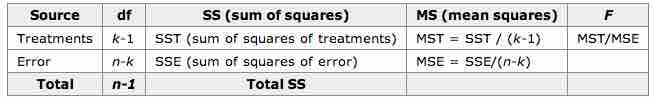
ANOVA Calculation Table
This table summarizes the calculations necessary in an ANOVA for comparing multiple means.
Letting
and the sum of the squares of the treatments is:
where
The sum of squares of the error SSE is given by:
and
Example
An example for the effect of breakfast on attention span (in minutes) for small children is summarized in the table below:
.
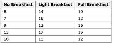
Breakfast and Children's Attention Span
This table summarizes the effect of breakfast on attention span (in minutes) for small children.
The hypothesis test would be:
versus:
The solution to the test can be seen in the figure below:
.
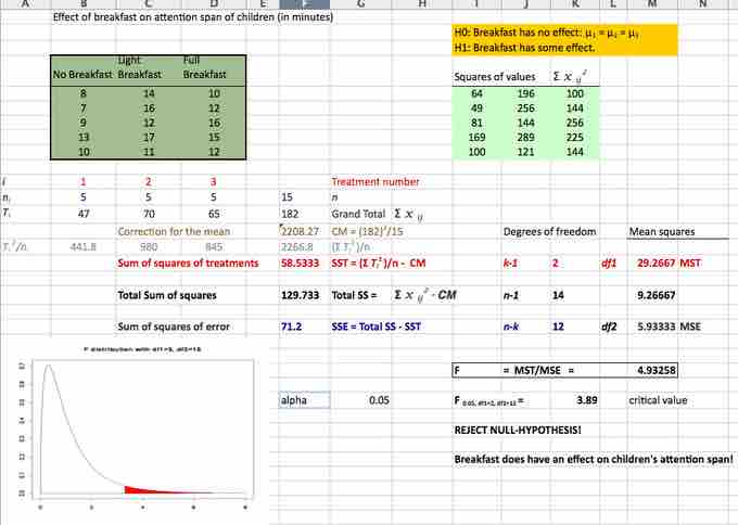
Excel Solution
This image shows the solution to our ANOVA example performed in Excel.
The test statistic
Hence, this indicates that the means are not equal (i.e., that sample values give sufficient evidence that not all means are the same). In terms of the example this means that breakfast (and its size) does have an effect on children's attention span.