Graphing the Normal Distribution

The graph of a normal distribution is a bell curve, as shown below.

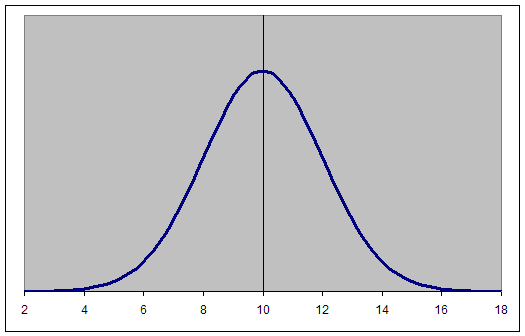
The Bell Curve

The graph of a normal distribution is known as a bell curve.

The properties of the bell curve are as follows.

• It is perfectly symmetrical.
• It is unimodal (has a single mode).
• Its domain is all real numbers.
• The area under the curve is 1.

Different values of the mean and standard deviation determine the density factor. Mean specifically determines the height of a bell curve, and standard deviation relates to the width or spread of the graph. The height of the graph at any $x$ value can be found through the equation:

$\displaystyle \frac{1}{\sigma\sqrt{2\pi}}e^{-\frac{1}{2}\left(\frac{x-\mu}{\sigma}\right)^2}$

In order to picture the value of the standard deviation of a normal distribution and it's relation to the width or spread of a bell curve, consider the following graphs. Out of these two graphs, graph 1 and graph 2, which one represents a set of data with a larger standard deviation?

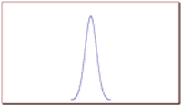
Graph 1

Bell curve visualizing a normal distribution with a relatively small standard deviation.

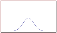
Graph 2

Bell curve visualizing a normal distribution with a relatively large standard deviation.

The correct answer is graph 2. The larger the standard deviation, the wider the graph. The smaller it is, the narrower the graph.

Percentiles and the Normal Curve

Percentiles represent the area under the normal curve, increasing from left to right. Each standard deviation represents a fixed percentile, and follows the empirical rule. Thus, rounding to two decimal places, $-3$ is the 0.13^th percentile, $-2$ the 2.28^th percentile, $-1$ the 15.87^th percentile, 0 the 50^th percentile (both the mean and median of the distribution), $+1$ the 84.13^th percentile, $+2$ the 97.72^nd percentile, and $+3$ the 99.87^th percentile. Note that the 0^th percentile falls at negative infinity and the 100^th percentile at positive infinity.