Statistics
Textbooks
Boundless Statistics
Continuous Random Variables
The Normal Curve
Statistics Textbooks Boundless Statistics Continuous Random Variables The Normal Curve
Statistics Textbooks Boundless Statistics Continuous Random Variables
Statistics Textbooks Boundless Statistics
Statistics Textbooks
Statistics
Concept Version 7
Created by Boundless

Continuous Probability Distributions

A continuous probability distribution is a representation of a variable that can take a continuous range of values.

Learning Objective

  • Explain probability density function in continuous probability distribution


Key Points

    • A probability density function is a function that describes the relative likelihood for a random variable to take on a given value.
    • Intuitively, a continuous random variable is the one which can take a continuous range of values — as opposed to a discrete distribution, where the set of possible values for the random variable is at most countable.
    • While for a discrete distribution an event with probability zero is impossible (e.g. rolling 3 and a half on a standard die is impossible, and has probability zero), this is not so in the case of a continuous random variable.

Term

  • Lebesgue measure

    The unique complete translation-invariant measure for the σ\sigmaσ-algebra which contains all kkk-cells—in and which assigns a measure to each kkk-cell equal to that kkk-cell's volume (as defined in Euclidean geometry: i.e., the volume of the kkk-cell equals the product of the lengths of its sides).


Full Text

A continuous probability distribution is a probability distribution that has a probability density function. Mathematicians also call such a distribution "absolutely continuous," since its cumulative distribution function is absolutely continuous with respect to the Lebesgue measure λ\lambdaλ. If the distribution of XXX is continuous, then XXX is called a continuous random variable. There are many examples of continuous probability distributions: normal, uniform, chi-squared, and others.

Intuitively, a continuous random variable is the one which can take a continuous range of values—as opposed to a discrete distribution, in which the set of possible values for the random variable is at most countable. While for a discrete distribution an event with probability zero is impossible (e.g. rolling 3 and a half on a standard die is impossible, and has probability zero), this is not so in the case of a continuous random variable.

For example, if one measures the width of an oak leaf, the result of 3.5 cm is possible; however, it has probability zero because there are uncountably many other potential values even between 3 cm and 4 cm. Each of these individual outcomes has probability zero, yet the probability that the outcome will fall into the interval (3 cm, 4 cm) is nonzero. This apparent paradox is resolved given that the probability that XXX attains some value within an infinite set, such as an interval, cannot be found by naively adding the probabilities for individual values. Formally, each value has an infinitesimally small probability, which statistically is equivalent to zero.

The definition states that a continuous probability distribution must possess a density; or equivalently, its cumulative distribution function be absolutely continuous. This requirement is stronger than simple continuity of the cumulative distribution function, and there is a special class of distributions—singular distributions, which are neither continuous nor discrete nor a mixture of those. An example is given by the Cantor distribution. Such singular distributions, however, are never encountered in practice.

Probability Density Functions

In theory, a probability density function is a function that describes the relative likelihood for a random variable to take on a given value. The probability for the random variable to fall within a particular region is given by the integral of this variable's density over the region. The probability density function is nonnegative everywhere, and its integral over the entire space is equal to one.

Unlike a probability, a probability density function can take on values greater than one. For example, the uniform distribution on the interval [0,12]\left[0, \frac{1}{2}\right][0,​2​​1​​] has probability density f(x)=2f(x) = 2f(x)=2 for 0≤x≤120 \leq x \leq \frac{1}{2}0≤x≤​2​​1​​ and f(x)=0f(x) = 0f(x)=0 elsewhere. The standard normal distribution has probability density function:

f(x)=12πe−12x2\displaystyle f(x) = \frac{1}{\sqrt{2\pi}}e^{-\frac{1}{2}x^2}f(x)=​√​2π​​​​​1​​e​−​2​​1​​x​2​​​​.

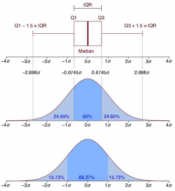
Boxplot Versus Probability Density Function

Boxplot and probability density function of a normal distribution N(0,2)N(0, 2)N(0,2).

[ edit ]
Edit this content
Prev Concept
The Hypergeometric Random Variable
The Uniform Distribution
Next Concept
Subjects
  • Accounting
  • Algebra
  • Art History
  • Biology
  • Business
  • Calculus
  • Chemistry
  • Communications
  • Economics
  • Finance
  • Management
  • Marketing
  • Microbiology
  • Physics
  • Physiology
  • Political Science
  • Psychology
  • Sociology
  • Statistics
  • U.S. History
  • World History
  • Writing

Except where noted, content and user contributions on this site are licensed under CC BY-SA 4.0 with attribution required.