Calculating a Normal Approximation

In this atom, we provide an example on how to compute a normal approximation for a binomial distribution.

Learning Objective

Demonstrate how to compute normal approximation for a binomial distribution

Key Points

In our example, we have a fair coin and wish to know the probability that you would get 8 heads out of 10 flips.
The binomial distribution has a mean of $\mu = Np = 10\cdot 0.5 = 5$ and a variance of $\sigma^2 = Np(1-p) = 10 \cdot 0.5\cdot 0.5 = 2.5$; therefore a standard deviation of 1.5811.
A total of 8 heads is 1.8973 standard deviations above the mean of the distribution.
Because the binomial distribution is discrete an the normal distribution is continuous, we round off and consider any value from 7.5 to 8.5 to represent an outcome of 8 heads.
Using this approach, we calculate the area under a normal curve (which will be the binomial probability) from 7.5 to 8.5 to be 0.044.

Terms

binomial distribution
the discrete probability distribution of the number of successes in a sequence of $n$ independent yes/no experiments, each of which yields success with probability $p$
z-score
The standardized value of observation $x$ from a distribution that has mean $\mu$ and standard deviation $\sigma$.

Full Text

The following is an example on how to compute a normal approximation for a binomial distribution.

Assume you have a fair coin and wish to know the probability that you would get 8 heads out of 10 flips. The binomial distribution has a mean of $\mu = Np = 10\cdot 0.5 = 5$ and a variance of $\sigma^2 = Np(1-p) = 10 \cdot 0.5\cdot 0.5 = 2.5$. The standard deviation is, therefore, 1.5811. A total of 8 heads is:

$\displaystyle \frac { 8-5 }{ 1.5811 } =1.8973$

Standard deviations above the mean of the distribution. The question then is, "What is the probability of getting a value exactly 1.8973 standard deviations above the mean?" You may be surprised to learn that the answer is 0 (the probability of any one specific point is 0). The problem is that the binomial distribution is a discrete probablility distribution whereas the normal distribultion is a continuous distribution.

The solution is to round off and consider any value from 7.5 to 8.5 to represent an outcome of 8 heads. Using this approach, we calculate the area under a normal curve from 7.5 to 8.5. The area in green in the figure is an approximation of the probability of obtaining 8 heads.

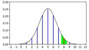
Normal Approximation

Approximation for the probability of 8 heads with the normal distribution.

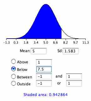
To calculate this area, first we compute the area below 8.5 and then subtract the area below 7.5. This can be done by finding $z$-scores and using the $z$-score table. Here, for the sake of ease, we have used an online normal area calculator. The results are shown in the following figures:

Normal Area 2

This graph shows the area below 7.5.

Normal Area 1

This graph shows the area below 8.5.

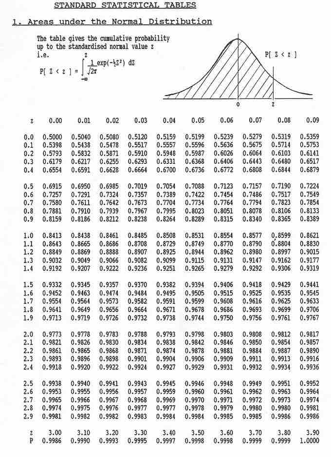
$z$-Score Table

The $z$-score table is used to calculate probabilities for the standard normal distribution.

The differences between the areas is 0.044, which is the approximation of the binomial probability. For these parameters, the approximation is very accurate. If we did not have the normal area calculator, we could find the solution using a table of the standard normal distribution (a $z$-table) as follows:

Find a $Z$ score for 7.5 using the formula $Z=\frac { 7.5-5 }{ 1.5811 } =1.5811$
Find the area below a $Z$ of $1.58=0.943$.
Find a $Z$ score for 8.5 using the formula $Z=\frac { 8.5-5 }{ 1.5811 } =2.21$
Find the area below a $Z$ of $2.21=0.987$.
Subtract the value in step 2 from the value in step 4 to get 0.044.

The same logic applies when calculating the probability of a range of outcomes. For example, to calculate the probability of 8 to 10 flips, calculate the area from 7.5 to 10.5.

[ edit ]

Prev Concept

The Scope of the Normal Approximation

Change of Scale

Next Concept