Polynomials appear in a wide variety of areas of mathematics and science. To better study and understand a polynomial, we sometimes like to draw its graph.

Visible Properties of a Polynomial

A typical graph of a polynomial function of degree 3 is the following:

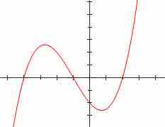
A polynomial of degree $3$

Graph of a polynomial function with equation $y = \frac {x^3}{4} + \frac {3x^2}{4} - \frac {3x}{2} - 2.$

Zeros

If we factorize the above function we see that $y = \frac{1}{4}(x-2)(x+1)(x+4)$, so the zeros of the polynomial are $2, -1$ and $-4$. This is one thing we can read from the graph. In general, we can read the number of zeros from a polynomial just by looking at how many times it meets the $x$-axis. 

Behavior Near Infinity

As $\frac {x^3}{4}$ tends to be much larger (in absolute value) than $\frac {3x^2}{4} - \frac {3x}{2} - 2$ when $x$ tends to positive or negative infinity, we see that $y$ goes, like $\frac {x^3}{4}$, to negative infinity when $x$ goes to negative infinity, and to positive infinity when $x$ goes to positive infinity. This is again something we can read from the graph. 

In general, polynomials will show the same behavior as their highest-degree term. Functions of even degree will go to positive or negative infinity (depending on the sign of the coefficient of the highest-degree term) if $x$ goes to infinity. Functions of odd degree will go to negative or positive infinity when $x$ goes to negative infinity and vice versa, again depending on the highest-degree term coefficient. 

How to Sketch a Graph

Conversely, if we know the zeros of a polynomial, and we know how it behaves near infinity, we can already make a nice sketch of the graph. We can exactly draw the points $(z,0)$ for each root $z$. Between two zeros (and before the smallest zero, and after the greatest zero) a function will always be either positive, or negative. We know whether it is positive or negative at infinity. Every time we cross a zero of odd multiplicity (if the number of zeros equals the degree of the polynomial, all zeros have multiplicity one and thus odd multiplicity) we change sign. 

So in our example, we start with a negative sign until we reach $x = -4$, when our graph rises above the $x$-axis. At some point it starts to descend again, until we reach $x=-1$ and the graph goes below the $x$-axis again till $x=2$, where it becomes positive again. 

With this procedure, we can draw a reasonable sketch of our graph, by only looking at the sign of the function and drawing a smooth line with the same sign! However, we can do better. For example, the number of times a function reaches a local minimum or maximum (i.e. a point where the graph descends and then starts to ascend again, or vice versa) is finite. In particular, it is smaller than the degree of the given polynomial. So if you draw a graph, make sure you draw no more local extremum points than you should. 

Easy Points to Draw

Another easy point to draw is the intersection with the $y$-axis, as this equals the function value in the point zero, which equals the constant term of the polynomial. We also call this the $y$-intercept of the function. So if we draw our smooth line, we make sure it crosses the $y$-axis in the same place. In general, the more function values we compute, the more points of the graph we know, and the more accurate our graph will be. Conversely, we can easily read the constant term of the polynomial by looking at its intersection with the $y$-axis if its graph is given (and indeed, we can readily read any function value if the graph is given). 

 Examples

• The graph of the zero polynomial $f(x)=0$ is the $x$-axis, since all real numbers are zeros. 
• The graph of a degree $0$ polynomial $f(x)=a_0$, where $a_0 \not = 0$, is a horizontal line with $y$-intercept $a_0$.
• The graph of a degree 1 polynomial (or linear function)$f(x) = a_0 + a_1x$, where $a_1 \not = 0$, is a straight line with $y$-intercept $a_0$ and slope $a_1$.
• The graph of a degree 2 polynomial $f(x) = a_0 + a_1x + a_2x^2$, where $a_2 \neq 0$ is a parabola.
• The graph of a degree 3 polynomial $f(x) = a_0 + a_1x + a_2x^2 + a_3x^3$, where $a_3 \neq 0$, is a cubic curve.
• The graph of any polynomial with degree 2 or greater $f(x) = a_0 + a_1x + a_2x^2 + ... + a_nx^n$, where $a_n \neq 0$ and $n \geq 2$ is a continuous non-linear curve.
• The graph of a non-constant (univariate) polynomial always tends to infinity when the variable increases indefinitely (in absolute value).

Examples

Below are some examples of graphs of functions. 

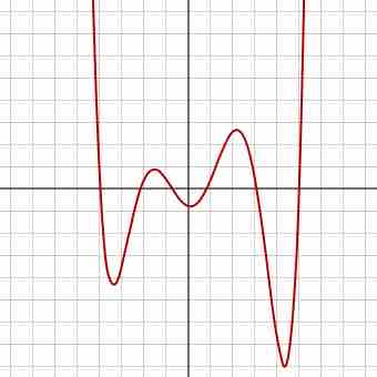
A polynomial of degree 6

A polynomial of degree 6. Its constant term is between -1 and 0. Its highest-degree coefficient is positive. It has exactly 6 zeroes and 5 local extrema.

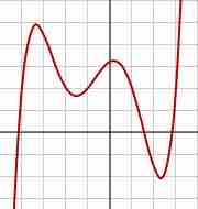
A polynomial of degree 5

A polynomial of degree 5. Its constant term is between 3 and 4. Its highest-degree coefficient is positive. It has 3 real zeros (and two complex ones). However, it has 4 local extrema.