Algebra
Textbooks
Boundless Algebra
Exponents, Logarithms, and Inverse Functions
Graphs of Exponential and Logarithmic Functions
Algebra Textbooks Boundless Algebra Exponents, Logarithms, and Inverse Functions Graphs of Exponential and Logarithmic Functions
Algebra Textbooks Boundless Algebra Exponents, Logarithms, and Inverse Functions
Algebra Textbooks Boundless Algebra
Algebra Textbooks
Algebra
Concept Version 11
Created by Boundless

Solving Problems with Logarithmic Graphs

Some functions with rapidly changing shape are best plotted on a scale that increases exponentially, such as a logarithmic graph.

Learning Objective

  • Discuss the advantages of using logarithmic scales for certain graphs


Key Points

    • Logarithmic graphs use logarithmic scales, in which the values differ exponentially. For example, instead of including marks at $0,1,2$ and $3$, a logarithmic scale may include marks at $0.1, 1, 10$ and $100$, each an equal distance from the previous and next.
    • Logarithmic graphs allow one to plot a very large range of data without losing the shape of the graph.
    • Logarithmic graphs make it easier to interpolate in areas that may be difficult to read on linear axes. For example, if the plot $y=x^5$ is scaled to show a very wide range of $y$ values, the curvature near the origin may be indistinguishable on linear axes. It is much clearer on logarithmic axes.

Terms

  • logarithm

    The logarithm of a number is the exponent by which another fixed value, the base, has to be raised to produce that number.

  • interpolate

    To estimate the value of a function between two points between which it is tabulated.


Full Text

Why Use a Logarithmic Scale?

Many mathematical and physical relationships are functionally dependent on high-order variables. This means that for small changes in the independent variable there are very large changes in the dependent variable. Thus, it becomes difficult to graph such functions on the standard axis.

Consider, as an example, the Stefan-Boltzmann law, which relates the power (j*) emitted by a black body to temperature (T).

$j^*= \sigma T^4$

On a standard graph, this equation can be quite unwieldy. The fourth-degree dependence on temperature means that power increases extremely quickly. The fact that the rate is ever-increasing (and steeply so) means that changing scale (scaling the axes by $5$, $10$ or even $100$) is of little help in making the graph easier to interpret.

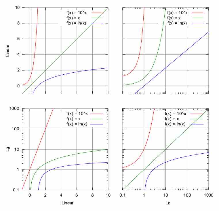
For very steep functions, it is possible to plot points more smoothly while retaining the integrity of the data: one can use a graph with a logarithmic scale . Here are some examples of functions graphed on a linear scale, semi-log and logarithmic scales. 

The top left is a linear scale. The bottom right is a logarithmic scale. The top right and bottom left are called semi-log scales because one axis is scaled linearly while the other is scaled using logarithms.

Logarithmic scale

The graphs of functions $f(x)=10^x,f(x)=x$ and $f(x)=\log x$ on four different coordinate plots. Top Left is a linear scale, top right and bottom left are semi-log scales and bottom right is a logarithmic scale.

As you can see, when both axis used a logarithmic scale (bottom right) the graph retained the properties of the original graph (top left) where both axis were scaled using a linear scale. That means that if we want to graph a function that is unwieldy on a linear scale we can use a logarithmic scale on each axis and retain the properties of the graph while at the same time making it easier to graph. 

It should be noted that the examples in the graphs were meant to illustrate a point and that the functions graphed were not necessarily unwieldy on a linearly scales set of axes.

Converting Linear to Logarithmic Scales

The primary difference between the logarithmic and linear scales is that, while the difference in value between linear points of equal distance remains constant (that is, if the space from $0$ to $1$ on the scale is $1$ cm on the page, the distance from $1$ to $2$, $2$ to $3$, etc., will be the same), the difference in value between points on a logarithmic scale will change exponentially. A logarithmic scale will start at a certain power of $10$, and with every unit will increase by a power of $10$.

Thus, if one wanted to convert a linear scale (with values $0-5$ to a logarithmic scale, one option would be to replace $1,2,3,4$ and 5 with $0.001,0.01,0.1,1,10$ and $100$, respectively. Between each major value on the logarithmic scale, the hashmarks become increasingly closer together with increasing value. For example, in the space between $1$ and $10$, the $8$ and $9$ are much closer together than the $2$ and $3$.

The advantages of using a logarithmic scale are twofold. Firstly, doing so allows one to plot a very large range of data without losing the shape of the graph. Secondly, it allows one to interpolate at any point on the plot, regardless of the range of the graph. Similar data plotted on a linear scale is less clear.

Solving Problems Using Logarithmic Graphs

A key point about using logarithmic graphs to solve problems is that they expand scales to the point at which large ranges of data make more sense. In the equation mentioned above ($j^*= \sigma T^4$), plotting $j$ vs. $T$ would generate the expected curve, but the scale would be such that minute changes go unnoticed and the large scale effects of the relationship dominate the graph: It is so big that the "interesting areas" won't fit on the paper on a readable scale.

Taking the logarithm of each side of the equations yields: $logj=log{(\sigma\tau ) }^4 $. We now rely on the properties of logarithms to re-write the equation. 

Recall the following properties of logarithms:

$\log(ab)=\log(a)+\log(b) \\ \log(a)^b=(b)\log(a)$

Using the above, our equation becomes: 

$\begin{aligned} \log j&=4\log{(\sigma\tau ) } \\ &=4\log{(\sigma)}+4\log{(\tau ) } \\ &=4\log{(\tau ) }+4\log{(\sigma)} \end{aligned} $

[ edit ]
Edit this content
Prev Concept
Graphs of Logarithmic Functions
Logarithms of Products
Next Concept
Subjects
  • Accounting
  • Algebra
  • Art History
  • Biology
  • Business
  • Calculus
  • Chemistry
  • Communications
  • Economics
  • Finance
  • Management
  • Marketing
  • Microbiology
  • Physics
  • Physiology
  • Political Science
  • Psychology
  • Sociology
  • Statistics
  • U.S. History
  • World History
  • Writing

Except where noted, content and user contributions on this site are licensed under CC BY-SA 4.0 with attribution required.