Statistics
Textbooks
Boundless Statistics
Correlation and Regression
The Regression Line
Statistics Textbooks Boundless Statistics Correlation and Regression The Regression Line
Statistics Textbooks Boundless Statistics Correlation and Regression
Statistics Textbooks Boundless Statistics
Statistics Textbooks
Statistics
Concept Version 7
Created by Boundless

Model Assumptions

Standard linear regression models with standard estimation techniques make a number of assumptions.

Learning Objective

  • Contrast standard estimation techniques for standard linear regression


Key Points

    • There are five major assumptions made by standard linear regression models.
    • The arrangement, or probability distribution, of the predictor variables $x$ has a major influence on the precision of estimates of $\beta$.
    • Extensions of the major assumptions make the estimation procedure more complex and time-consuming, and may even require more data in order to get an accurate model.

Term

  • exogeneity

    a condition in linear regression wherein the variable is independent of all other response values


Full Text

Standard linear regression models with standard estimation techniques make a number of assumptions about the predictor variables, the response variables, and their relationship. Numerous extensions have been developed that allow each of these assumptions to be relaxed (i.e. reduced to a weaker form), and in some cases eliminated entirely. Some methods are general enough that they can relax multiple assumptions at once, and in other cases this can be achieved by combining different extensions. Generally, these extensions make the estimation procedure more complex and time-consuming, and may even require more data in order to get an accurate model.

The following are the major assumptions made by standard linear regression models with standard estimation techniques (e.g. ordinary least squares):

Weak exogeneity. This essentially means that the predictor variables $x$ can be treated as fixed values rather than random variables. This means, for example, that the predictor variables are assumed to be error-free; that is, they are not contaminated with measurement errors. Although unrealistic in many settings, dropping this assumption leads to significantly more difficult errors-in-variables models.

Linearity. This means that the mean of the response variable is a linear combination of the parameters (regression coefficients) and the predictor variables. Note that this assumption is far less restrictive than it may at first seem. Because the predictor variables are treated as fixed values (see above), linearity is really only a restriction on the parameters. The predictor variables themselves can be arbitrarily transformed, and in fact multiple copies of the same underlying predictor variable can be added, each one transformed differently. This trick is used, for example, in polynomial regression, which uses linear regression to fit the response variable as an arbitrary polynomial function (up to a given rank) of a predictor variable. This makes linear regression an extremely powerful inference method. In fact, models such as polynomial regression are often "too powerful" in that they tend to overfit the data. As a result, some kind of regularization must typically be used to prevent unreasonable solutions coming out of the estimation process.

Constant variance (aka homoscedasticity). This means that different response variables have the same variance in their errors, regardless of the values of the predictor variables. In practice, this assumption is invalid (i.e. the errors are heteroscedastic) if the response variables can vary over a wide scale. In order to determine for heterogeneous error variance, or when a pattern of residuals violates model assumptions of homoscedasticity (error is equally variable around the 'best-fitting line' for all points of $x$), it is prudent to look for a "fanning effect" between residual error and predicted values. This is to say there will be a systematic change in the absolute or squared residuals when plotted against the predicting outcome. Error will not be evenly distributed across the regression line. Heteroscedasticity will result in the averaging over of distinguishable variances around the points to get a single variance that is inaccurately representing all the variances of the line. In effect, residuals appear clustered and spread apart on their predicted plots for larger and smaller values for points along the linear regression line, and the mean squared error for the model will be wrong. Typically, for example, a response variable whose mean is large will have a greater variance than one whose mean is small.

Independence of errors. This assumes that the errors of the response variables are uncorrelated with each other. (Actual statistical independence is a stronger condition than mere lack of correlation and is often not needed, although it can be exploited if it is known to hold. ) Some methods (e.g. generalized least squares) are capable of handling correlated errors, although they typically require significantly more data unless some sort of regularization is used to bias the model towards assuming uncorrelated errors. Bayesian linear regression is a general way of handling this issue.

Lack of multicollinearity in the predictors. For standard least squares estimation methods, the design matrix $X$ must have full column rank $p$; otherwise, we have a condition known as multicollinearity in the predictor variables. This can be triggered by having two or more perfectly correlated predictor variables (e.g. if the same predictor variable is mistakenly given twice, either without transforming one of the copies or by transforming one of the copies linearly). It can also happen if there is too little data available compared to the number of parameters to be estimated (e.g. fewer data points than regression coefficients). Beyond these assumptions, several other statistical properties of the data strongly influence the performance of different estimation methods:

The statistical relationship between the error terms and the regressors plays an important role in determining whether an estimation procedure has desirable sampling properties such as being unbiased and consistent.

The arrangement, or probability distribution, of the predictor variables $x$ has a major influence on the precision of estimates of $\beta$. Sampling and design of experiments are highly-developed subfields of statistics that provide guidance for collecting data in such a way as to achieve a precise estimate of $\beta$.

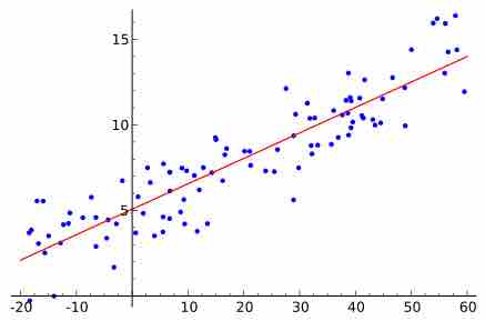
Simple Linear Regression

A graphical representation of a best fit line for simple linear regression.

[ edit ]
Edit this content
Prev Concept
Least-Squares Regression
Making Inferences About the Slope
Next Concept
Subjects
  • Accounting
  • Algebra
  • Art History
  • Biology
  • Business
  • Calculus
  • Chemistry
  • Communications
  • Economics
  • Finance
  • Management
  • Marketing
  • Microbiology
  • Physics
  • Physiology
  • Political Science
  • Psychology
  • Sociology
  • Statistics
  • U.S. History
  • World History
  • Writing

Except where noted, content and user contributions on this site are licensed under CC BY-SA 4.0 with attribution required.