Calculus
Textbooks
Boundless Calculus
Differential Equations, Parametric Equations, and Sequences and Series
Differential Equations
Calculus Textbooks Boundless Calculus Differential Equations, Parametric Equations, and Sequences and Series Differential Equations
Calculus Textbooks Boundless Calculus Differential Equations, Parametric Equations, and Sequences and Series
Calculus Textbooks Boundless Calculus
Calculus Textbooks
Calculus
Concept Version 8
Created by Boundless

Direction Fields and Euler's Method

Direction fields and Euler's method are ways of visualizing and approximating the solutions to differential equations.

Learning Objective

  • Describe application of direction fields and Euler's method to approximate the solutions to differential equations


Key Points

    • Direction fields, or slope fields, are graphs where each point $(x,y)$ has a slope.
    • Euler's method is a way of approximating solutions to differential equations by assuming that the slope at a point is the same as the slope between that point and the next point.
    • Euler's method gives approximate solutions to differential equations, and the smaller the distance between the chosen points, the more accurate the result.

Terms

  • differential equation

    an equation involving the derivatives of a function

  • tangent

    a straight line touching a curve at a single point without crossing it there

  • normalize

    (in mathematics) to divide a vector by its magnitude to produce a unit vector


Full Text

Direction Fields

Direction fields, also known as slope fields, are graphical representations of the solution to a first order differential equation. They can be achieved without solving the differential equation analytically, and serve as a useful way to visualize the solutions.

The slope field is traditionally defined for differential equations of the following form:

 $y'=f(x)$

It can be viewed as a creative way to plot a real-valued function of two real variables as a planar picture.
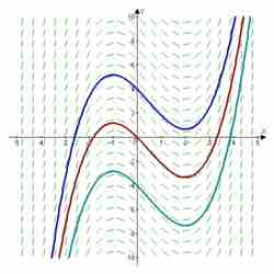
Example slope field

The slope field of $\frac{dy}{dx}=x^2-x-2$, with the blue, red, and turquoise lines being $\frac{x^3}{3}-\frac{x^2}{2}-2x+4$, $\frac{x^3}{3}-\frac{x^2}{2}-2x$, and $\frac{x^3}{3}-\frac{x^2}{2}-2x-4$, respectively.

Specifically, for a given pair, a vector with the components is drawn at the point $(x,y)$ on the $xy$-plane. Sometimes, the vector is normalized to make the plot more pleasing to the human eye. A set of pairs $(x,y)$ making a rectangular grid is typically used for the drawing. An isocline (a series of lines with the same slope) is often used to supplement the slope field. In an equation of the form, the isocline is a line in the $xy$-plane obtained by setting $f(x,y)$ equal to a constant.

Euler's Method

Consider the problem of calculating the shape of an unknown curve which starts at a given point and satisfies a given differential equation. Here, a differential equation can be thought of as a formula by which the slope of the tangent line to the curve can be computed at any point on the curve, once the position of that point has been calculated.The idea is that while the curve is initially unknown, its starting point, which we denote by
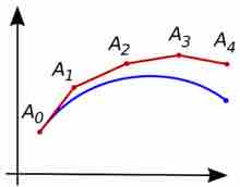
 $A_0$, is known (see ). Then, from the differential equation, the slope to the curve at $A_0$ can be computed, and thus, the tangent line.

Euler's Method

Illustration of the Euler method. The unknown curve is in blue and its polygonal approximation is in red.

Take a small step along that tangent line up to a point, $A_1$. Along this small step, the slope does not change too much $A_1$ will be close to the curve. If we pretend that $A_1$ is still on the curve, the same reasoning we used for the above point, $A_0$, can be applied. After several steps, a polygonal curve is computed. In general, this curve does not diverge too far from the original unknown curve, and the error between the two curves can be made small if the step size is small enough and the interval of computation is finite.

[ edit ]
Edit this content
Prev Concept
Models Using Differential Equations
Separable Equations
Next Concept
Subjects
  • Accounting
  • Algebra
  • Art History
  • Biology
  • Business
  • Calculus
  • Chemistry
  • Communications
  • Economics
  • Finance
  • Management
  • Marketing
  • Microbiology
  • Physics
  • Physiology
  • Political Science
  • Psychology
  • Sociology
  • Statistics
  • U.S. History
  • World History
  • Writing

Except where noted, content and user contributions on this site are licensed under CC BY-SA 4.0 with attribution required.