Curve Fitting
Curve fitting is the process of constructing a curve, or mathematical function, that has the best fit to a series of data points, possibly subject to constraints. Curve fitting can involve either interpolation, where an exact fit to the data is required, or smoothing, in which a "smooth" function is constructed that approximately fits the data. Fitted curves can be used as an aid for data visualization, to infer values of a function where no data are available, and to summarize the relationships among two or more variables. Extrapolation refers to the use of a fitted curve beyond the range of the observed data, and is subject to a greater degree of uncertainty since it may reflect the method used to construct the curve as much as it reflects the observed data.
In this section, we will only be fitting lines to data points, but it should be noted that one can fit polynomial functions, circles, piece-wise functions, and any number of functions to data and it is a heavily used topic in statistics.
Linear Regression Formula
Linear regression is an approach to modeling the linear relationship between a dependent variable,
The simplest and perhaps most common linear regression model is the ordinary least squares approximation. This approximation attempts to minimize the sums of the squared distance between the line and every point.
To find the slope of the line of best fit, calculate in the following steps:
- The sum of the product of the
$x$ and$y$ coordinates$\sum_{i=1}^{n}x_{i}y_{i}$ . - The sum of the
$x$ -coordinates$\sum_{i=1}^{n}x_{i}$ . - The sum of the
$y$ -coordinates$\sum_{j=1}^{n}y_{j}$ . - The sum of the squares of the
$x$ -coordinates$\sum_{i=1}^{n}(x_{i}^{2})$ . - The sum of the
$x$ -coordinates squared$(\sum_{i=1}^{n}x_{i})^{2}$ . - The quotient of the numerator and denominator.
To find the
- The average of the
$y$ -coordinates. Let$\bar{y}$ , pronounced$y$ -bar, represent the mean (or average)$y$ value of all the data points:$\bar y =\frac{1}{n}\sum_{i=1}^{n} y_{i}$ . - The average of the
$x$ -coordinates. Respectively$\bar{x}$ , pronounced$x$ -bar, is the mean (or average)$x$ value of all the data points:$\bar x=\frac{1}{n}\sum_{i=1}^{n} x_{i}$ . - Replace values into the formula above
$b=\bar{y} - m \bar{x}$ .
Using these values of
Using the Least Squares Approximation
Example: Write the least squares fit line and then graph the line that best fits the data
For
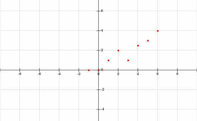
Example Points
The points are graphed in a scatterplot fashion.
First, find the slope
To find the slope, calculate:
- The sum of the product of the
$x$ and$y$ coordinates$\sum_{i=1}^{n}x_{i}y_{i}$ . - The sum of the
$x$ -coordinates$\sum_{i=1}^{n}x_{i}$ . - The sum of the
$y$ -coordinates$\sum_{i=1}^{n}y_{i}$ .
4. Calculate the numerator: The product of the
The numerator in the slope equation is:
5. Calculate the denominator: The
sum of the squares of the
The denominator is
Now for the
Therefore
Our final equation is therefore

Least Squares Fit Line
The line found by the least squares approximation,
Outliers and Least Square Regression
If we have a point that is far away from the approximating line, then it will skew the results and make the line much worse. For instance, let's say in our original example, instead of the point
Using the same calculations as above with the new point, the results are:
Looking at the points and line in the new figure below, this new line does not fit the data well, due to the outlier
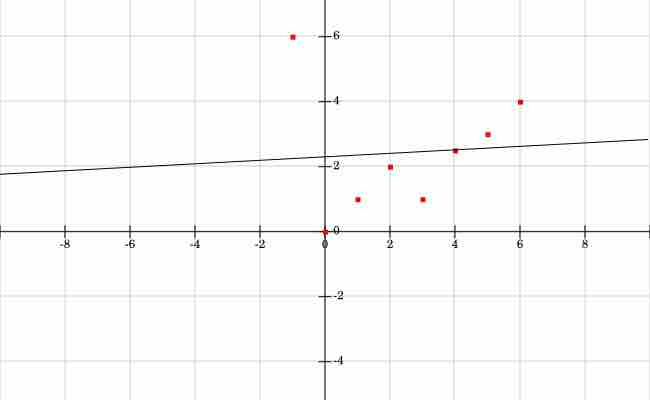
Outlier Approximated Line
Here is the approximated line given the new outlier point at (-1, 6).