The Binomial Formula

The binomial distribution is a discrete probability distribution of the successes in a sequence of $n$ independent yes/no experiments.

Learning Objective

Employ the probability mass function to determine the probability of success in a given amount of trials

Key Points

The probability of getting exactly $k$ successes in $n$ trials is given by the Probability Mass Function.
The binomial distribution is frequently used to model the number of successes in a sample of size $n$ drawn with replacement from a population of size $N$ .
The binomial distribution is the discrete probability distribution of the number of successes in a sequence of $n$ independent yes/no experiments, each of which yields success with probability $p$ .

Terms

probability mass function
a function that gives the probability that a discrete random variable is exactly equal to some value
central limit theorem
a theorem which states that, given certain conditions, the mean of a sufficiently large number of independent random variables--each with a well-defined mean and well-defined variance-- will be approximately normally distributed

Example

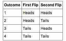
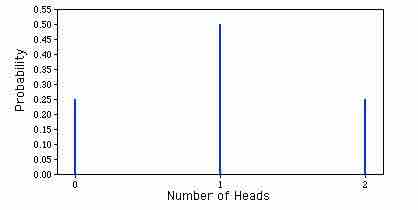
The four possible outcomes that could occur if you flipped a coin twice are listed in Table 1. Note that the four outcomes are equally likely: each has probability of $\frac{1}{4}$ . To see this, note that the tosses of the coin are independent (neither affects the other). Hence, the probability of a head on flip one and a head on flip two is the product of $P(H)$ and $P(H)$ , which is $\frac{1}{2} \cdot \frac{1}{2} = \frac{1}{4}$ . The same calculation applies to the probability of a head on flip one and a tail on flip two. Each is $\frac{1}{2} \cdot \frac{1}{2} = \frac{1}{4}$ . The four possible outcomes can be classified in terms of the number of heads that come up. The number could be two (Outcome 1), one (Outcomes 2 and 3) or 0 (Outcome 4). The probabilities of these possibilities are shown in Table 2 and in Figure 1. Since two of the outcomes represent the case in which just one head appears in the two tosses, the probability of this event is equal to $\frac{1}{4} + \frac{1}{4} = \frac{1}{2}$ . Table 1 summarizes the situation. Table 1 is a discrete probability distribution: It shows the probability for each of the values on the $x$ -axis. Defining a head as a "success," Table 1 shows the probability of 0, 1, and 2 successes for two trials (flips) for an event that has a probability of 0.5 of being a success on each trial. This makes Table 1 an example of a binomial distribution.

Full Text

In probability theory and statistics, the binomial distribution is the discrete probability distribution of the number of successes in a sequence of $n$ independent yes/no experiments, each of which yields success with probability $p$ . The binomial distribution is the basis for the popular binomial test of statistical significance.

Binomial Probability Distribution

This is a graphic representation of a binomial probability distribution.

The binomial distribution is frequently used to model the number of successes in a sample of size $n$ drawn with replacement from a population of size $N$ . If the sampling is carried out without replacement, the draws are not independent and so the resulting distribution is a hypergeometric distribution, not a binomial one. However, for $N$ much larger than $n$ , the binomial distribution is a good approximation, and widely used.

In general, if the random variable $X$ follows the binomial distribution with parameters $n$ and $p$ , we write $X \sim B(n, p)$ . The probability of getting exactly $k$ successes in $n$ trials is given by the Probability Mass Function:

$\displaystyle f(k; n, p) = P(X=k) = {{n}\choose{k}}p^k(1-p)^{n-k}$

For $k = 0, 1, 2, \dots, n$ where:

$\displaystyle {{n}\choose{k}} = \frac{n!}{k!(n-k)!}$

Is the binomial coefficient (hence the name of the distribution) "n choose k," also denoted $C(n, k)$ or $_nC_k$ . The formula can be understood as follows: We want $k$ successes ( $p^k$ ) and $n-k$ failures ( $(1-p)^{n-k}$ ); however, the $k$ successes can occur anywhere among the $n$ trials, and there are $C(n, k)$ different ways of distributing $k$ successes in a sequence of $n$ trials.

One straightforward way to simulate a binomial random variable $X$ is to compute the sum of $n$ independent 0−1 random variables, each of which takes on the value 1 with probability $p$ . This method requires $n$ calls to a random number generator to obtain one value of the random variable. When $n$ is relatively large (say at least 30), the Central Limit Theorem implies that the binomial distribution is well-approximated by the corresponding normal density function with parameters $\mu = np$ and $\sigma = \sqrt{npq}$ .

Figures from the Example

Table 1

These are the four possible outcomes from flipping a coin twice.

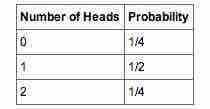
Table 2

These are the probabilities of the 2 coin flips.

[ edit ]

Prev Concept

Expected Values of Discrete Random Variables

Binomial Probability Distributions

Next Concept