Statistics
Textbooks
Boundless Statistics
Probability and Variability
Discrete Random Variables
Statistics Textbooks Boundless Statistics Probability and Variability Discrete Random Variables
Statistics Textbooks Boundless Statistics Probability and Variability
Statistics Textbooks Boundless Statistics
Statistics Textbooks
Statistics
Concept Version 10
Created by Boundless

Probability Distributions for Discrete Random Variables

Probability distributions for discrete random variables can be displayed as a formula, in a table, or in a graph.

Learning Objective

  • Give examples of discrete random variables


Key Points

    • A discrete probability function must satisfy the following: 0≤f(x)≤10 \leq f(x) \leq 10≤f(x)≤1, i.e., the values of f(x)f(x)f(x) are probabilities, hence between 0 and 1.
    • A discrete probability function must also satisfy the following: ∑f(x)=1\sum f(x) = 1∑f(x)=1, i.e., adding the probabilities of all disjoint cases, we obtain the probability of the sample space, 1.
    • The probability mass function has the same purpose as the probability histogram, and displays specific probabilities for each discrete random variable. The only difference is how it looks graphically.

Terms

  • probability mass function

    a function that gives the relative probability that a discrete random variable is exactly equal to some value

  • discrete random variable

    obtained by counting values for which there are no in-between values, such as the integers 0, 1, 2, ….

  • probability distribution

    A function of a discrete random variable yielding the probability that the variable will have a given value.


Full Text

A discrete random variable xxx has a countable number of possible values. The probability distribution of a discrete random variable xxx lists the values and their probabilities, where value x1x_1x​1​​ has probability p1p_1p​1​​, value x2x_2x​2​​ has probability x2x_2x​2​​, and so on. Every probability pip_ip​i​​ is a number between 0 and 1, and the sum of all the probabilities is equal to 1.

Examples of discrete random variables include:

  • The number of eggs that a hen lays in a given day (it can't be 2.3)
  • The number of people going to a given soccer match
  • The number of students that come to class on a given day
  • The number of people in line at McDonald's on a given day and time

A discrete probability distribution can be described by a table, by a formula, or by a graph. For example, suppose that xxx is a random variable that represents the number of people waiting at the line at a fast-food restaurant and it happens to only take the values 2, 3, or 5 with probabilities 210\frac{2}{10}​10​​2​​,  310\frac{3}{10}​10​​3​​, and 510\frac{5}{10}​10​​5​​ respectively. This can be expressed through the function f(x)=x10f(x)= \frac{x}{10}f(x)=​10​​x​​, x=2,3,5x=2, 3, 5x=2,3,5 or through the table below. Of the conditional probabilities of the event BBB given that A1A_1A​1​​ is the case or that A2A_2A​2​​ is the case, respectively. Notice that these two representations are equivalent, and that this can be represented graphically as in the probability histogram below.

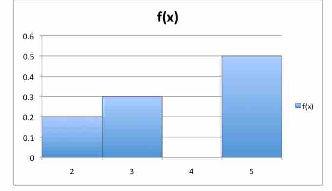
Probability Histogram

This histogram displays the probabilities of each of the three discrete random variables.

The formula, table, and probability histogram satisfy the following necessary conditions of discrete probability distributions:

  1. 0≤f(x)≤10 \leq f(x) \leq 10≤f(x)≤1, i.e., the values of f(x)f(x)f(x) are probabilities, hence between 0 and 1.
  2. ∑f(x)=1\sum f(x) = 1∑f(x)=1, i.e., adding the probabilities of all disjoint cases, we obtain the probability of the sample space, 1.

Sometimes, the discrete probability distribution is referred to as the probability mass function (pmf). The probability mass function has the same purpose as the probability histogram, and displays specific probabilities for each discrete random variable. The only difference is how it looks graphically.

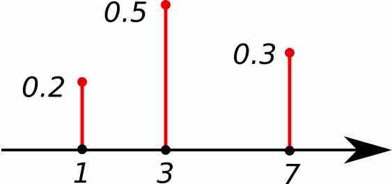
Probability Mass Function

This shows the graph of a probability mass function. All the values of this function must be non-negative and sum up to 1.

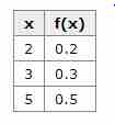
Discrete Probability Distribution

This table shows the values of the discrete random variable can take on and their corresponding probabilities.

[ edit ]
Edit this content
Prev Concept
Two Types of Random Variables
Expected Values of Discrete Random Variables
Next Concept
Subjects
  • Accounting
  • Algebra
  • Art History
  • Biology
  • Business
  • Calculus
  • Chemistry
  • Communications
  • Economics
  • Finance
  • Management
  • Marketing
  • Microbiology
  • Physics
  • Physiology
  • Political Science
  • Psychology
  • Sociology
  • Statistics
  • U.S. History
  • World History
  • Writing

Except where noted, content and user contributions on this site are licensed under CC BY-SA 4.0 with attribution required.