Statistics
Textbooks
Boundless Statistics
Continuous Random Variables
Normal Approximation
Statistics Textbooks Boundless Statistics Continuous Random Variables Normal Approximation
Statistics Textbooks Boundless Statistics Continuous Random Variables
Statistics Textbooks Boundless Statistics
Statistics Textbooks
Statistics
Concept Version 7
Created by Boundless

The Normal Approximation to the Binomial Distribution

The process of using the normal curve to estimate the shape of the binomial distribution is known as normal approximation.

Learning Objective

  • Explain the origins of central limit theorem for binomial distributions


Key Points

    • Originally, to solve a problem such as the chance of obtaining 60 heads in 100 coin flips, one had to compute the probability of 60 heads, then the probability of 61 heads, 62 heads, etc, and add up all these probabilities.
    • Abraham de Moivre noted that when the number of events (coin flips) increased, the shape of the binomial distribution approached a very smooth curve.
    • Therefore, de Moivre reasoned that if he could find a mathematical expression for this curve, he would be able to solve problems such as finding the probability of 60 or more heads out of 100 coin flips much more easily.
    • This is exactly what he did, and the curve he discovered is now called the normal curve.

Terms

  • normal approximation

    The process of using the normal curve to estimate the shape of the distribution of a data set.

  • central limit theorem

    The theorem that states: If the sum of independent identically distributed random variables has a finite variance, then it will be (approximately) normally distributed.


Full Text

The binomial distribution can be used to solve problems such as, "If a fair coin is flipped 100 times, what is the probability of getting 60 or more heads?" The probability of exactly xxx heads out of NNN flips is computed using the formula:

P(x)=N!x!(N−x)!πx(1−π)N−x\displaystyle P\left( x \right) =\frac { N! }{ x!\left( N-x \right) ! } { \pi }^{ x }{ \left( 1-\pi \right) }^{ N-x }P(x)=​x!(N−x)!​​N!​​π​x​​(1−π)​N−x​​

where xxx is the number of heads (60), NNN is the number of flips (100), and π\piπ is the probability of a head (0.5). Therefore, to solve this problem, you compute the probability of 60 heads, then the probability of 61 heads, 62 heads, etc, and add up all these probabilities.

Abraham de Moivre, an 18th century statistician and consultant to gamblers, was often called upon to make these lengthy computations. de Moivre noted that when the number of events (coin flips) increased, the shape of the binomial distribution approached a very smooth curve. Therefore, de Moivre reasoned that if he could find a mathematical expression for this curve, he would be able to solve problems such as finding the probability of 60 or more heads out of 100 coin flips much more easily. This is exactly what he did, and the curve he discovered is now called the normal curve. The process of using this curve to estimate the shape of the binomial distribution is known as normal approximation.

Normal Approximation

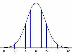
The normal approximation to the binomial distribution for 12 coin flips. The smooth curve is the normal distribution. Note how well it approximates the binomial probabilities represented by the heights of the blue lines.

The importance of the normal curve stems primarily from the fact that the distribution of many natural phenomena are at least approximately normally distributed. One of the first applications of the normal distribution was to the analysis of errors of measurement made in astronomical observations, errors that occurred because of imperfect instruments and imperfect observers. Galileo in the 17th century noted that these errors were symmetric and that small errors occurred more frequently than large errors. This led to several hypothesized distributions of errors, but it was not until the early 19th century that it was discovered that these errors followed a normal distribution. Independently the mathematicians Adrian (in 1808) and Gauss (in 1809) developed the formula for the normal distribution and showed that errors were fit well by this distribution.

This same distribution had been discovered by Laplace in 1778—when he derived the extremely important central limit theorem. Laplace showed that even if a distribution is not normally distributed, the means of repeated samples from the distribution would be very nearly normal, and that the the larger the sample size, the closer the distribution would be to a normal distribution. Most statistical procedures for testing differences between means assume normal distributions. Because the distribution of means is very close to normal, these tests work well even if the distribution itself is only roughly normal.

[ edit ]
Edit this content
Prev Concept
Finding the Area Under the Normal Curve
The Scope of the Normal Approximation
Next Concept
Subjects
  • Accounting
  • Algebra
  • Art History
  • Biology
  • Business
  • Calculus
  • Chemistry
  • Communications
  • Economics
  • Finance
  • Management
  • Marketing
  • Microbiology
  • Physics
  • Physiology
  • Political Science
  • Psychology
  • Sociology
  • Statistics
  • U.S. History
  • World History
  • Writing

Except where noted, content and user contributions on this site are licensed under CC BY-SA 4.0 with attribution required.