Google Sheets

Introduction

After you've added a lot of content to a spreadsheet, it can sometimes be difficult to view and read all of your information easily. Formatting allows you to customize the look and feel of your spreadsheet, making it easier to view and understand.

In this lesson, you'll learn how to modify the size, style, and color of text in your cells. You will also learn how to set text alignments and how to add borders and background colors to your cells.

Formatting cells

Video: Formatting Cells

Watch the video (3:54).

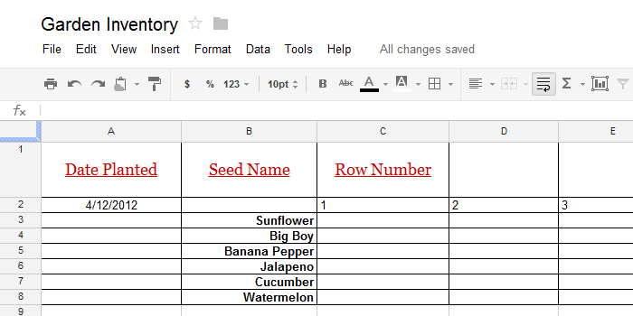
Every cell in a new spreadsheet uses the same default formatting. As you begin to build a spreadsheet, you can customize the formatting to make your information easier to view and understand. In our example, we will be using a spreadsheet to plan and organize a garden plot.

To change the font size:

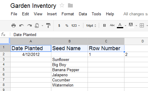
Modifying the font size can help call attention to important cells and make them easier to read. In our example, we will be increasing the size of our header cells to help distinguish them from the rest of the spreadsheet.

1. Select the cell or cells you wish to modify.
   
   Selecting the desired cells
2. Locate and select the Font Size button in the shortcut toolbar, then choose the desired font size from the drop-down menu. In our example, we will choose 14pt to make the text larger.
   
   Changing the font size
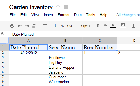
3. The text will change to the new font size.
   
   The updated font size

To change the font:

While Google Spreadsheets does not offer many choices, choosing a different font can help to further separate certain parts of your spreadsheet, like the header cells, from the rest of your information.

1. Select the cell or cells you wish to modify.
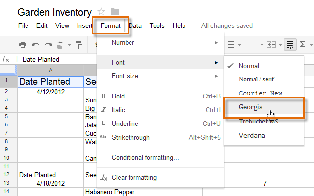
2. Locate and select Format in the toolbar menu.
3. Hover the mouse over Font, then select a new font from the drop-down menu. In our example, we will select Georgia.
   
   Changing the font style
4. The text will change to the new font.
   
   The new font style

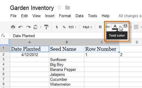
To change the text color:

1. Select the cell or cells you wish to modify.
2. Locate and select the Text color button in the shortcut toolbar.
   Changing the text color
3. A drop-down menu of different text colors will appear.
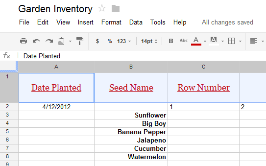
4. Select the color you wish to use. In our example, we will select red.
   
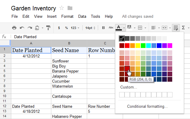   Choosing a text color
5. The text will change to the new color.
   
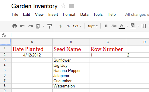   The new text color

To make text bold:

1. Select the text you wish to modify.
2. To bold text, click the Bold text button or press Ctrl+B (Windows) or Command+B (Mac) on your keyboard.
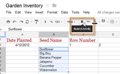   Bolding text
3. The text will change to bold.
   
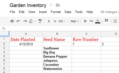   The bolded text

Press Ctrl+I (Windows) or Command+I (Mac) on your keyboard to add italics. Press Ctrl+U (Windows) or Command+U (Mac) to add underlining.

Italics and underlining

Text alignment

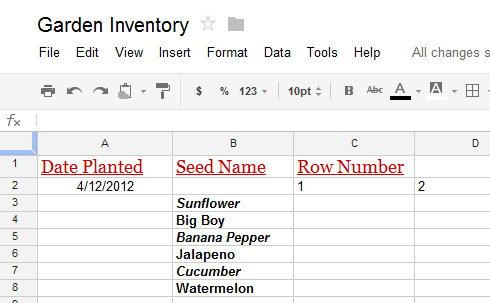
By default, any text entered into your spreadsheet will be aligned to the bottom-left of a cell. Any numbers will be aligned to the bottom-right of a cell. Changing the alignment of your cell content allows you to choose where the content will appear in any cell.

To modify the horizontal text alignment:

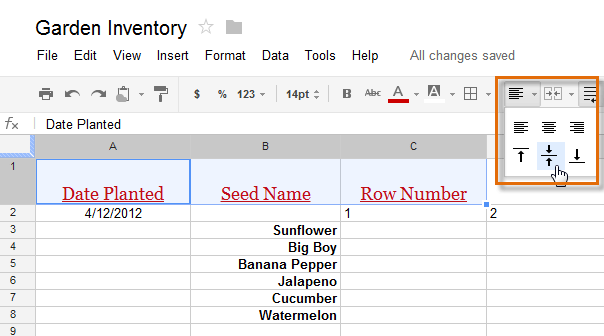
1. Select the text you wish to modify, then click the Align button in the shortcut toolbar.
   
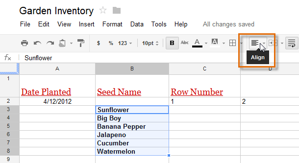   Clicking the Align button
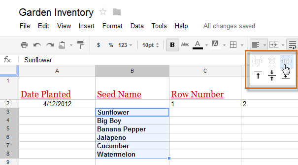
2. Select the desired alignment from the top of the drop-down menu.
   • Left align: Aligns content to the left border of the cell
   • Center align: Aligns content an equal distance from the left and right borders of the cell
   • Right align: Aligns content to the right border of the cell
   Choosing the horizontal alignment
3. The text will realign.
   
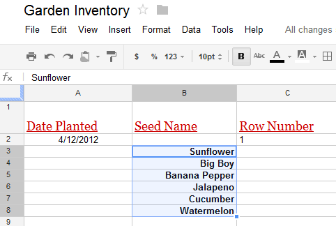   The new horizontal alignment

To modify the vertical text alignment:

1. Select the text you wish to modify, then click the Align button in the shortcut toolbar.
2. Choose the desired alignment from the drop-down menu.
   • Top align: Aligns content to the top border of the cell
   • Center align: Aligns content an equal distance from the top and bottom borders of the cell
   • Bottom align: Aligns content to the bottom border of the cell
   Choosing the vertical alignment
3. The text will realign.
   
   The new vertical alignment

You can apply both vertical and horizontal alignment settings to any cell.

Cell borders and background colors

Cell borders and background colors make it easy to create clear and defined boundaries for different sections of your spreadsheet.

To add cell borders:

1. Select the cell or cells you wish to modify.
2. Locate and select the Borders button from the shortcut toolbar.
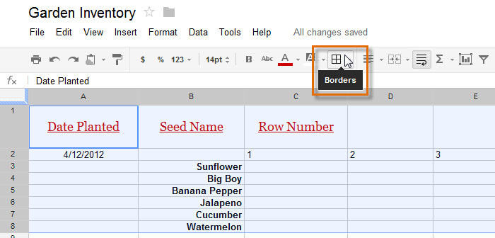   Clicking the Borders button
3. Choose the desired border option from the drop-down menu. In our example, we will choose to display all cell borders .
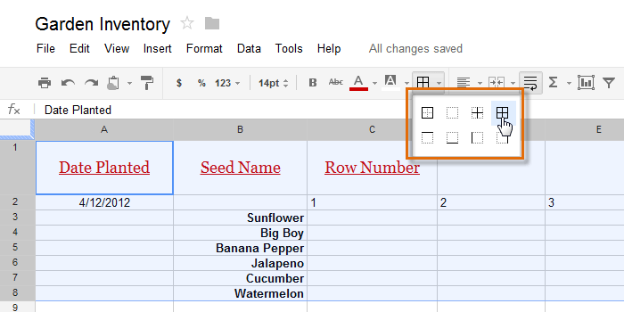   Selecting the cell border settings
4. The new cell borders will appear.
   
   The new cell borders

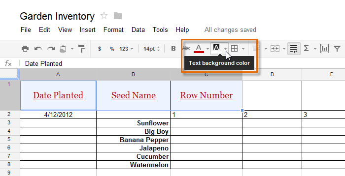
To change the text background color:

It's easy to change the background color of any cell, which is known as the text background color.

1. Select the cell or cells you wish to modify.
2. Locate and select the Fill button from the shortcut toolbar.
   Changing the text background color
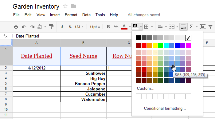
3. Select a color from the drop-down menu. In our example, we'll choose blue.
   
   Choosing a text background color
4. The new text background color will appear.
   
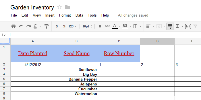   The new text background color

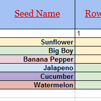
You can also use text background color to represent different kinds of information. In our example below, each seed planted in the garden is represented by a different background color.

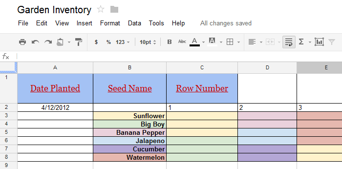Cells with multiple background colors

Formatting text and numbers

The ability to apply specific formatting for text and numbers is one of the most powerful tools in Google Spreadsheets. Instead of displaying all cell content in exactly the same way, you can use formatting to change the appearance of dates, times, decimals, percentages (%), currency ($), and much more.

To applying number formatting:

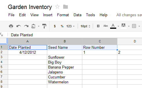
1. Select the cell or cells you wish to modify. In our example, we will change the date formatting of cell A2.
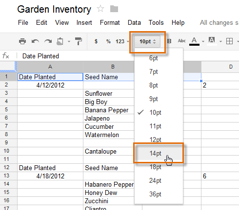
2. Locate and select the Number Formatting button from the shortcut toolbar.
   
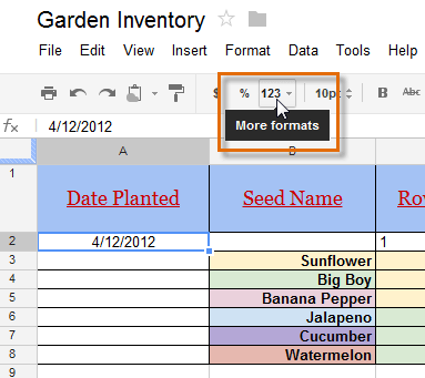   Adding number formatting
3. A drop-down menu will appear with various number formatting options.
4. Select the desired formatting. In our example, we will select a different type of date formatting.
   
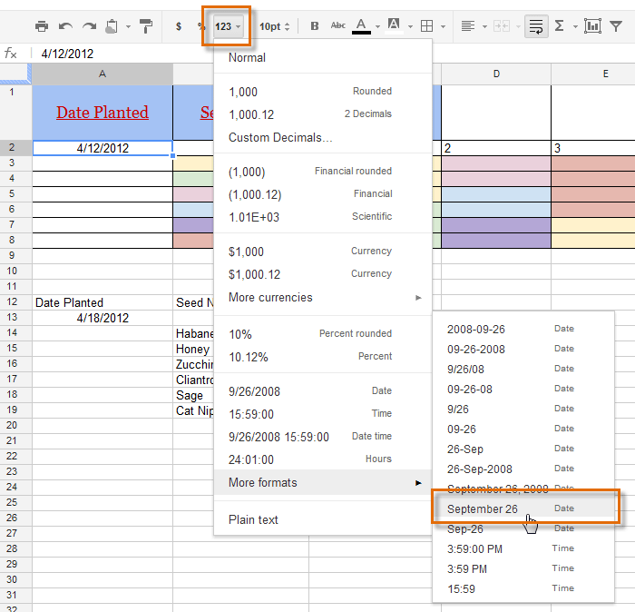   Choosing a format
5. The cell will change to the new formatting style.
   
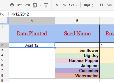   The formatted cell

Click the buttons in the interactive below to more learn about text and number formatting.

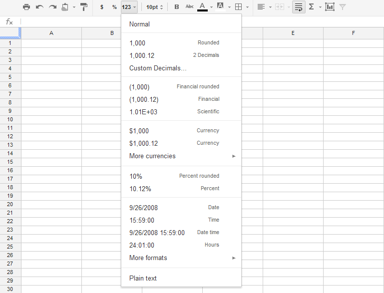
Normal Formatting

Normal is the default setting for every cell in a spreadsheet.

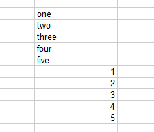
Whenver you enter information into a cell, Google Spreadsheets will choose a formatting style based on the content.

By default, text wil be left-aligned and numbers will be right-aligned.

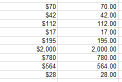
Decimals

Select 2 Decimals to round a decimal to the nearest hundredth (18.16).

Select Rounded to round a decimal to the nearest whole number (18).

These two options are used to simplify decimals in our example below.

Click Custom Decimals... to choose specific rounding for decimals.

Financial

Select Financial to format numbers for accounting purposes.

Select this option when working with a large amount of financial information.

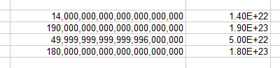
Scientific

Select Scientific to format numbers in scientific notation. This is especially helpful when working with very large numbers. In our example, the large numbers followed by many zeros are changed to the shorter, scientific format: 1.40E+22, 1.90E+23, and so on.

By default, Google Spreadsheets will apply scientific formatting if a number is too large to display in a cell.

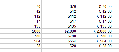
Currency

Select Currency to add proper puncuation and currency symbols, like the dollar sign ($), to numerical values.

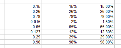
Percentages

Select Percent to add the Percent sign (%) to numerical values.

Percentages can be formatted in two different ways: as Percent rounded (15%) and as exact percet (15.00%).

In our example below, we have forrmatted the same percentages using these options

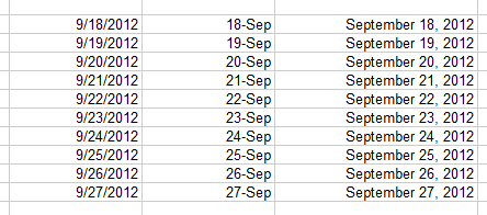
Time and Date

There are numerous options for formatting time and date in your spreadsheet.

In our example below, we have applied three different formats to the same dates.

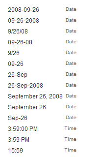
More Date and Time Formats

Hover the mouse over More formats to see more time and date options.

Plain Text

Select Plain text to remove all formatting from your cell content.

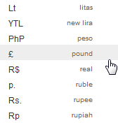
More Currency Formats

Hover the mouse over More Currencies to see more international currency options.

If you're using the new Google Sheets, you may notice that the number formatting options have changed. For more information about the new options, check out our lesson on Understanding the New Google Sheets.

Challenge!

To work through the challenge, open GCFLearnFree L10: Garden Inventory and copy the file to your Google Drive. View the instructions below the challenge if you are not sure how to make a copy of the file.

1. Increase the font size of cell G1 to 14pt.
2. Change the font style of cells B3:B8 to Verdana.
3. Select a new font color for cell G1.
4. Modify the horizontal alignment of cells B3:B8 to center align.
5. Add borders to cells B1:G8.
6. Set a different text background color for each day in cells G3:G8.

To copy the example file to your Google Drive:

In these tutorials, we will provide example files you can use to practice what you've learned in each lesson. Because these files are Google Docs we have chosen to share, you will need to copy the file to your Google Drive before you can edit the file.

1. Click the link at the top of this page to open the example file.
2. The example file will appear in a new browser tab or window. If you are not currently signed in to your Google account, locate and click Sign in on the top-right corner of the page.
   
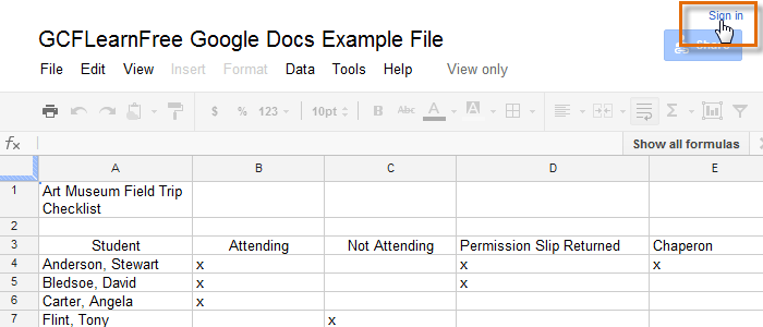   Signing in to your Google Account
3. After you have signed in to your Google account, locate and select File in the toolbar menu, then select Make a copy... from the drop-down menu.
   
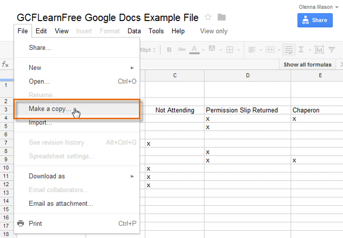   Making a copy of the example file
4. The Copy Document dialog box will appear. Enter a new title for the file, then click OK.
   
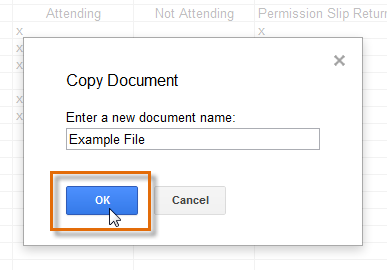   Naming the file and clicking OK
5. The copy of the file will appear in a new browser tab. Now you're ready to start using the example file.
   
   Viewing the copied example file in a new tab